Predict detection probability at given distance

Eric Rexstad

CREEM, Univ of St Andrews

December 2024

Motivation

Having fitted a detection function model to distance sampling data, often there is interest in using the fitted model to predict detection probability for combinations of predictors (including distance).

Commonly this is done when covariates other that distance are included in the model. For example, researchers may want to know the difference in predicted detection probability at a given distance among different habitat types. It is this scenario that lead to the development of this case study. Credit to Ward Langeraert for bringing this to our attention.

We construct a simple simulated line transect distance sampling survey, sampling a population consisting of four types: two sexes and two ages. Each of the four categories of animals have distinct simulated detection functions. We generate a single survey of this population and fit a detection function containing an agesex covariate, consistent with how the simulated data were generated.

The main focus of this case study is interrogating the fitted model to a) visualise the fitted detection function model for each of the four age/sex classes and b) focus upon the differences in predicted detection probability between age/sex classes at a specified perpendicular distance. However, the application of the approach demonstrated in this case study is not limited only to those situations.

Simulate a data set

The simulation of a data set is accomplished using the dsims package Marshall (2024). Details of the dsims package will not be described here, interested readers should follow the previous link.

library(dsims)

## Loading required package: dssd

set.seed(19511)
study.region <- make.region()
density <- make.density(region = study.region)
covariate.list <- list()
# The population equal proportion in four age/sex classes
covariate.list$agesex <- list(data.frame(level = c("youngmale", "youngfemale", "adultmale", "adultfemale"), 
                                          prob = rep(0.25,4)))
pop.desc <- make.population.description(region = study.region, 
                                        density = density, 
                                        N = 400,
                                        covariates = covariate.list,
                                        fixed.N = TRUE)
cov.params <- list()
truncation_distance <- 50
cov.params$agesex = data.frame(level = c("youngmale", "youngfemale", "adultmale", "adultfemale"), 
                            param = c(0.2, 0.7, 1.0, 1.3))
detect.cov <- make.detectability(key.function = "hn" ,
                                 scale.param = 10,
                                 cov.param = cov.params, 
                                 truncation = truncation_distance)
plot(detect.cov, pop.desc, lwd=3)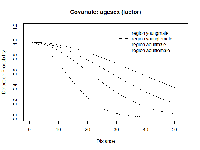

Figure 1: Simulated detection functions for four age x sex classes.

design <- make.design(region = study.region,
                      transect.type = "line",
                      design = "systematic",
                      spacing = 100,
                      truncation = truncation_distance)
analysis.cov <- make.ds.analysis(dfmodel = list(~agesex),
                                 key = "hn",
                                 truncation = truncation_distance)
my.simulation <- make.simulation(reps = 999, 
                                 design = design,
                                 population.description = pop.desc,
                                 detectability = detect.cov,
                                 ds.analysis = analysis.cov)
my.survey <- run.survey(my.simulation)
ds_model <- analyse.data(analysis.cov, my.survey)

The plot created in the above chunk shows the simulated detection functions for each age/sex class in the simulated population. The last object created in the above chunk is of type dsmodel, equivalent to objects created by the ds() function in the Distance package. It is this object (ds_model) that you would have created in your analysis and want to use to predict detection probabilities from the fitted model.

Interrogate ds_model$ddf

To produce our predicted detection probabilities, we need merely one component of the ds_model object. It is called ddfobj and it is located deep within ds_model, specificially ds_model$ddf$ds$aux$ddfobj

The function that does the work of producing estimated detection probabilities from a ddfobj along with a detection distance and an index to the set of predictor covariates is called detfct in the mrds package.

Code below isolated the ddfobj within ds_model just to make life easier. Then the index of the first observation of each age/sex combination is found within the design matrix (because the design matrix is formed after any truncation takes place in model fitting).

ddfobj <- ds_model$ddf$ds$aux$ddfobj
ym.indx <- which(ddfobj$xmat$agesex=="youngmale")[1]
yf.indx <- which(ddfobj$xmat$agesex=="youngfemale")[1]
am.indx <- which(ddfobj$xmat$agesex=="adultmale")[1]
af.indx <- which(ddfobj$xmat$agesex=="adultfemale")[1]

This completes the preliminaries to use detfct for predicting detection probabilities.

Predict detection probability at a specific distance

The next code chunk uses detfct to predict detection probabilities for each age/sex class at a single perpendicular distance.

mydist <- 35
Young_male <- mrds::detfct(mydist, ddfobj, index = ym.indx)
Young_female <- mrds::detfct(mydist, ddfobj, index = yf.indx)
Adult_male <- mrds::detfct(mydist, ddfobj, index = am.indx)
Adult_female <- mrds::detfct(mydist, ddfobj, index = af.indx)
outtable <- data.frame(Age_sex_class=c("Young male", "Young female", "Adult male", "Adult female"),
                       Predicted_p=c(Young_male, Young_female, Adult_male, Adult_female))
knitr::kable(outtable, digits = 3, 
             caption="Predicted detection probabilities at 35m")

Table 1: Predicted detection probabilities at 35m

Age_sex_class	Predicted_p
Young male	0.014
Young female	0.059
Adult male	0.555
Adult female	0.439

Compute detection probabilities at range of distances

We will create a code chunk that duplicates the capability of the add_df_covar_line function found in the mrds package. The code plots a detection function for each of the four age/sex classes over a range of requested distances using the indices calculated in the previous chunk.

prediction_distances <- seq(0, 50) 
g_x_ym <- mrds::detfct(prediction_distances, ddfobj, index = ym.indx)
g_x_yf <- mrds::detfct(prediction_distances, ddfobj, index = yf.indx)
g_x_am <- mrds::detfct(prediction_distances, ddfobj, index = am.indx)
g_x_af <- mrds::detfct(prediction_distances, ddfobj, index = af.indx)

The vectors of predicted detection probabilities are plotted in the following chunk. The last section of the chunk adds the calculated probabilities at the 35m distance to the plot.

plot(ds_model, pl.col="white", cex=0.7)
lines(prediction_distances, g_x_ym, col="darkgreen", lwd=2)
lines(prediction_distances, g_x_yf, col = "green", lwd=2)
lines(prediction_distances, g_x_am, col = "darkblue", lwd=2)
lines(prediction_distances, g_x_af, col = "brown", lwd=2)
legend("topright", title="Age/sex class", lwd=2,
       legend=c("young male", "young female", "adult male", "adult female"),
       col=c("darkgreen", "green", "darkblue", "brown"))
#----------
abline(v=mydist, lwd=3)
segments(0, Young_male, mydist, Young_male, col="darkgreen")
segments(0, Young_female, mydist, Young_female, col="green")
segments(0, Adult_male, mydist, Adult_male, col="darkblue")
segments(0, Adult_female, mydist, Adult_female, col="brown")
text(0, Young_male, round(Young_male,3), adj=c(-.1, -.3), cex=0.7)
text(0, Young_female, round(Young_female,3), adj=c(-.1, -.3), cex=0.7)
text(0, Adult_male, round(Adult_male,3), adj=c(-.1, -.3), cex=0.7)
text(0, Adult_female, round(Adult_female,3), adj=c(-.1, -.3), cex=0.7)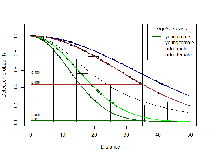

Figure 2: Predicted detection probabilities for four age x sex classes; with those at 35m highlighted.

Marshall, L. (2024). Dsims: Distance sampling simulations. Retrieved from https://github.com/DistanceDevelopment/dsims