Getting Started with dsims
L. Marshall
CREEM, Univ of St AndrewsSeptember 2025
Source:vignettes/GettingStarted.Rmd
GettingStarted.RmdDistance Sampling Simulations
This vignette introduces the basic procedure for setting up and running a distance sampling simulation using ‘dsims’ (Laura Marshall 2023a). The ‘dsims’ package uses the distance sampling survey design package ‘dssd’ (Laura Marshall 2023b) to define the design and generate the surveys (sets of transects). For further details on defining designs please refer to the ‘dssd’ vignettes. ‘dsims’ was designed to be largely similar to the ‘DSsim’ package (L. Marshall 2020) in terms of work flow, functions and arguments. The main differences in terms of its use lie in the definition of the designs which can now be generated in R using the ‘dssd’ package (these packages are automatically linked) and the definition of analyses. Analyses are now defined using terminology based on the ‘Distance’ package (Miller et al. 2019). In addition, the underlying functionality now makes use of the ‘sf’ package (Pebesma and Baston 2021).
Distance Sampling techniques provide design based estimates of density and abundance for populations. The accuracy of these estimates relies on valid survey design. While general rules of thumb can help guide our design choices, simulations emulating a specific set of survey characteristics can often help us achieve more efficient and robust designs for individual studies. For example, simulations can help us investigate how effort allocation can affect our estimates or the effects of a more efficient design which has less uniform coverage probability. Due to the individual nature of each study, each with their specific set of characteristics, simulation can be a powerful tool in evaluating survey design.
Setting up the Region
We will use the St Andrews bay area as an example study region for these simulations. This is a single strata study region which has been projected into metres. We will first load the ‘dsims’ package, this will also automatically load the ‘dssd’ package. As this shapefile does not have a projection recorded (in an associated .prj file) we tell ‘dsims’ that the units are metres.
## Loading required package: dssd
# Find the file path to the example shapefile in dssd
shapefile.name <- system.file("extdata", "StAndrew.shp", package = "dssd")
# Create the survey region object
region <- make.region(region.name = "St Andrews bay",
                      shape = shapefile.name,
                      units = "m")
plot(region)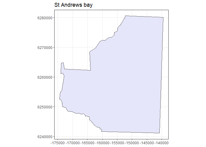
Figure 1: The study region.
Defining the study population
To define a study population we require a number of intermediate steps. We describe these in turn below.
Population Density Grid
The first step in defining your study population is to set up the density grid. One way to do this is to first create a flat surface and then add hot and low spots to represent where you think you might have areas of higher and lower density of animals.
If we were to assume that there were 300 groups in the St Andrews bay study area (which is a fairly large number!) this would only give us an average density of 3.04-07 groups per square metre. For this simulation, as we will use a fixed population size, we do not need to worry about the absolute values of the density surface. Instead, it can be simpler to work with larger values and be aware that we are defining a relative density surface. So where we create a surface to have a density of twice that in another area that relationship will be maintained (be it at much smaller absolute values) when we later generate the population.
For the purposes of simulation you will likely want to test over a range of plausible animal distributions (if you knew exactly how many you were going to find at any given location you probably wouldn’t be doing the study!). When testing non-uniform coverage designs it is advisable to try out worst case scenarios, i.e. set density in the area of higher or lower coverage to differ from the majority of the survey region. This will give an idea of the degree of potential bias which could be introduced.
In this example, for the equal spaced zigzag design, as it is generated in a convex hull the areas with differing coverage are likely to be at the very top and very bottom of the survey region. In the density grid below these areas are shown to have lower animal density than the rest of the survey region, a likely scenario when a study region has been constructed in order to catch the range of a population of interest.
# We first create a flat density grid
density <- make.density(region = region,
                        x.space = 500,
                        constant = 1)

# Now we can add some high and low points to give some spatial variability
density <- add.hotspot(object = density,
                       centre = c(-170000, 6255000),
                       sigma = 8000,
                       amplitude = 4)

density <- add.hotspot(object = density,
                       centre = c(-160000, 6275000),
                       sigma = 6000,
                       amplitude = 4)

density <- add.hotspot(object = density,
                       centre = c(-155000, 6260000),
                       sigma = 3000,
                       amplitude = 2)

density <- add.hotspot(object = density,
                       centre = c(-150000, 6240000),
                       sigma = 10000,
                       amplitude = -0.9)

density <- add.hotspot(object = density,
                       centre = c(-155000, 6285000),
                       sigma = 10000,
                       amplitude = -1)

# I will choose to plot in km rather than m (scale = 0.001)
plot(density, region, scale = 0.001)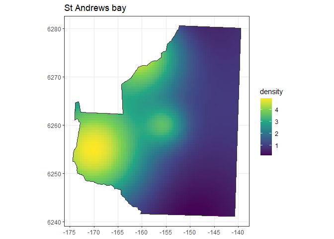
Figure 2: A density map representing a plausible distributions of animals within the study region.
In some situations you may not need to rely on constructing a density distribution from scratch. Now we will demonstrate how to use a gam to construct the density surface. As I do not have data for this area I will use the density grid I created above as an example dataset. I will fit a gam to this data and then use this to create a new density object. As I need to restrict the predicted values to be greater than zero, I will use a log link with the Gaussian error distribution. This can also be a useful trick if you want to turn something created using the above method, which can look a bit lumpy and bumpy, into a smoother distribution surface. The gam fitted must only use a smooth over x and y to fit the model as no other predictor covariates will be present in the density surface.
# First extract the data above - this is simple in this case as we only have a single strata
# Multi-strata regions will involve combining the density grids for each strata into a
# single dataset.
density.data <- density@density.surface[[1]]
head(density.data)
## Simple feature collection with 6 features and 4 fields
## Geometry type: POLYGON
## Dimension: XY
## Bounding box: xmin: -157572.4 ymin: 6241463 xmax: -154890.4 ymax: 6241543
## CRS: NA
## strata density x y geometry
## 34 St Andrews bay 0.6128054 -157640.4 6241293 POLYGON ((-157390.4 6241543...
## 35 St Andrews bay 0.5614958 -157140.4 6241293 POLYGON ((-157390.4 6241543...
## 36 St Andrews bay 0.5125986 -156640.4 6241293 POLYGON ((-156890.4 6241543...
## 37 St Andrews bay 0.4662975 -156140.4 6241293 POLYGON ((-156390.4 6241543...
## 38 St Andrews bay 0.4227525 -155640.4 6241293 POLYGON ((-155890.4 6241543...
## 39 St Andrews bay 0.3821010 -155140.4 6241293 POLYGON ((-155390.4 6241543...
# Fit a simple gam to the data
library(mgcv)
## Loading required package: nlme## This is mgcv 1.9-3. For overview type 'help("mgcv-package")'.
fit.gam <- gam(density ~ s(x,y), data = density.data, family = gaussian(link="log"))

# Use the gam object to create a density object
gam.density <- make.density(region = region,
                            x.space = 500,
                            fitted.model = fit.gam)

plot(gam.density, region, scale = 0.001)
Figure 3: A density map representing a plausible distributions of animals within the study region.
Other Population Parameters
Once we have created a plausible animal density distribution we can go on to define other population parameters. We do this by constructing a population description.
We will assume animals occur in small clusters so we will first create a covariate list and define the distribution for cluster size (which must be named “size”) as a zero-truncated Poisson distribution with mean equal to 3. For those of you familiar with ‘DSsim’ please note the simplified format for defining population covariates.
The other population value we have to define is the population size. As we have clusters in our population, N will refer to the number of clusters rather than individuals. We will set the number of clusters to be 100. We then leave the fixed.N argument as the default TRUE to say we would like to generate the population based on the population size rather than the density surface.
# Create a covariate list describing the distribution of cluster sizes
covariates <- list(size = list(distribution = "ztruncpois", mean = 3))

# Define the population description
pop.desc <- make.population.description(region = region,
                                        density = gam.density,
                                        covariates = covariates,
                                        N = 300,
                                        fixed.N = TRUE)
Coverage Grid
It is good practice to create a coverage grid over your study area to assess how coverage probability varies spatially across your study area for any specified designs. For designs where there may be non-uniform coverage, we advise coverage probability is assessed prior to running any simulations. However, as this step is not essential for running simulations we will omit it here and refer you to the ‘dssd’ vignettes for further details.
Defining the Design
‘dsims’ working together with ‘dssd’ provides a number of point and line transect designs. Further details on defining designs can be found in the ‘dssd’ help and vignettes. We also provide examples online at https://distancedevelopment.github.io/distancesamplingcom2/resources/vignettes.html .
For these simulations we will compare two line transect designs, systematically spaced parallel lines and equal spaced zigzag lines. The zigzag design will be generated within a convex hull to try to minimise the off-effort transit time between the ends of transects.
The design angles for each design were selected so that the transects run roughly perpendicular to the coast. The way the two designs are defined means that this is 90 degrees for the parallel line design and 0 for the zigzag design. Both designs assumed a minus sampling protocol and the truncation distance was set at 750m from the transect. The spacings for each design were selected to give the same trackline lengths of around 450 km (this was assessed by running the coverage simulations for these designs using ‘run.coverage’, see help in ‘dssd’). The trackline lengths can be thought of as an indicator of the cost of the survey as they give the total travel time (both on and off effort) from the beginning of the first transect to the end of the last transect.
parallel.design <- make.design(region = region,
                               design = "systematic",
                               spacing = 2500,
                               edge.protocol = "minus",
                               design.angle = 90,
                               truncation = 750)

zigzag.design <- make.design(region = region,
                             design = "eszigzag",
                             spacing = 2233,
                             edge.protocol = "minus",
                             design.angle = 0,
                             bounding.shape = "convex.hull",
                             truncation = 750)
Generating a Set of Transects
It is always a good idea to run a quick check that your design is as expected by generating a set of transects and plotting them.
p.survey <- generate.transects(parallel.design)
plot(region, p.survey)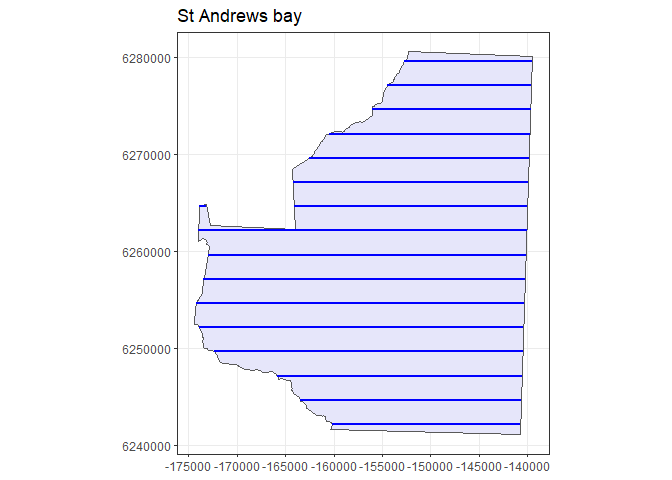
Figure 4: An example set of transects generated from the systematic parallel line design plotted within the study region.
z.survey <- generate.transects(zigzag.design)
plot(region, z.survey)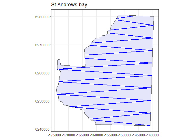
Figure 5: An example set of transects generated from the systematic parallel line design plotted within the study region.
Defining Detectability
Once we have defined both the population of interest and the design which we will use to survey our population we now need to provide information about how detectable the individuals or clusters are. For this example we will assume that larger clusters are more detectable. Take care when defining covariate parameters that the covariate names match those in the population description.
When setting the basic scale parameter along side covariate parameters values we need be aware of how the covariate parameter values are incorporated. The covariate parameter values provided adjust the value of the scale parameter on the log scale. The scale parameter for any individual (\(\sigma_j\)) can be calculated as:
\[\sigma_j = exp(log(\sigma_0)+\sum_{i=1}^{k}\beta_ix_{ij})\] where \(j\) is the individual, \(\sigma_0\) is the base line scale parameter (passed in as argument ‘scale.param’ on the natural scale), the \(\beta_i\)’s are the covariate parameters passed in on the log scale for each covariate \(i\) and the \(x_{ij}\) values are the covariate values for covariate \(i\) and individual \(j\).
We will assume a half normal detection function with a scale parameter of 300. We will set the truncation distance to be the same as the design at 750 m. and set the covariate slope coefficient on the log scale to log(1.08) = 0.077. We can check what our detection functions will look like for the different covariate values by plotting them. To plot the example detection functions we need to provide the population description as well as detectability.
# Define the covariate parameters on the log scale
cov.param <- list(size = log(1.08))

# Create the detectability description
detect <- make.detectability(key.function = "hn",
                             scale.param = 300,
                             cov.param = cov.param,
                             truncation = 750)

# Plot the simulation detection functions
plot(detect, pop.desc)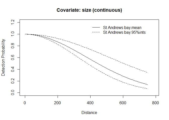
Figure 6: Plot of the detection function for the mean group size (solid line) and for the 2.5 and 97.5 percentile values of group size (dashed lines) for this population.
We can also calculate the average detection function for our mean cluster size of 3 as defined in our population description:
\[\sigma_{size = 3} = exp(log(300)+log(1.05)*3) = 347.3 \]
Defining Analyses
The final component to a simulation is the analysis or set of analyses you wish to fit to the simulated data. We will define a number of models and allow automatic model selection based on the minimum AIC value. The models included below are a half-normal with no covariates, a hazard rate with no covariates and a half-normal with cluster size as a covariate. We will leave the truncation value at 750 as previously defined (it must be \(\le\) to the truncation values used previously). We will use the default error variance estimator “R2”. See ?mrds::varn for descriptions of the various empirical variance estimators for encounter rate.
analyses <- make.ds.analysis(dfmodel = list(~1, ~1, ~size),
                             key = c("hn", "hr", "hn"),
                             truncation = 750,
                             er.var = "R2",
                             criteria = "AIC")
Putting the Simulation Together
Now we have all the simulation components defined we can create our simulation objects. We will create one for the systematic parallel line design and one for the equal spaced zigzag design.
sim.parallel <- make.simulation(reps = 999,
                                design = parallel.design,
                                population.description = pop.desc,
                                detectability = detect,
                                ds.analysis = analyses)

sim.zigzag <- make.simulation(reps = 999,
                              design = zigzag.design,
                              population.description = pop.desc,
                              detectability = detect,
                              ds.analysis = analyses)
Once you have created a simulation we recommend you check to see what a simulated survey might look like.
# Generate a single instance of a survey: a population, set of transects
# and the resulting distance data
eg.parallel.survey <- run.survey(sim.parallel)

# Plot it to view a summary
plot(eg.parallel.survey, region)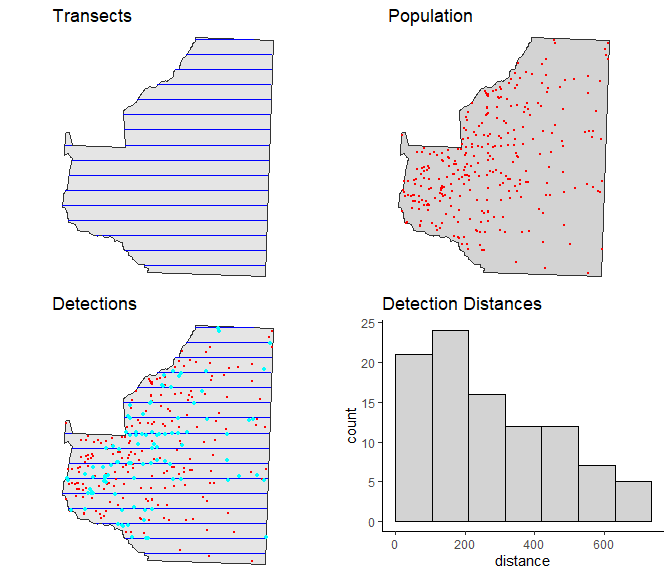
Figure 7: Example survey from systematic parallel design. Panels showing: top left - transects, top right - population, bottom left - transects, population and survey detections (cyan dots), bottom right - histogram of detection distances
# Generate a single instance of a survey: a population, set of transects
# and the resulting distance data
eg.zigzag.survey <- run.survey(sim.zigzag)

# Plot it to view a summary
plot(eg.zigzag.survey, region)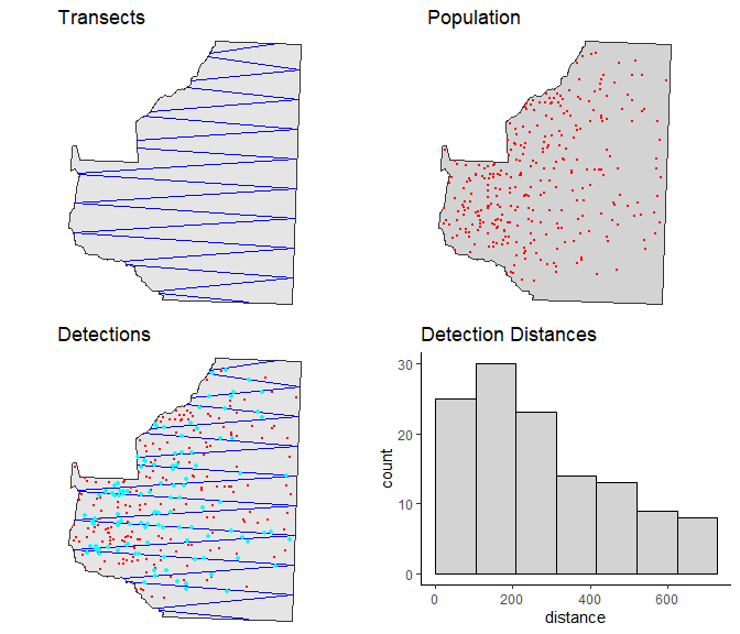
Figure 8: Example survey from equal spaced zigzag design. Panels showing: top left - transects, top right - population, bottom left - transects, population and survey detections (cyan dots), bottom right - histogram of detection distances
Running the Simulation
The simulations can be run as follows. Note that these will take some time to run!
# Running the simulations
sim.parallel <- run.simulation(sim.parallel)
sim.zigzag <- run.simulation(sim.zigzag)
Simulation Results
Once the simulations have run we can view a summary of the results. Viewing a summary of a simulation will first summarise the simulation setup and then if the simulation has been run provide a summary of the results. A glossary is also provided to aid interpretation of the results. Note that each run will produce slightly different results due to the random component of the generation of both the populations and the sets of survey transects.
Firstly, for the systematic parallel lines design we can see that there is very low bias 1.85% for the estimated abundance/density of individuals. The bias is even lower at only 0.16% for the estimated abundance/density of clusters. Also we can see that the analyses have done a good job at estimating the mean cluster size, there is only 1.72% bias.
We can also see that the 95% confidence intervals calculated for the abundance/density estimates are in fact capturing the true value around 97% of the time (CI.coverage.prob). We can also note that the observed standard deviation of the estimates of the mean is a bit lower than the mean se, meaning we are realising a lower variance than we would estimate. This is often seen with systematic designs as the default variance estimator assumes a completely random allocation of transect locations, systematic designs usually have lower variance.
Reassuringly, these results are as expected for the systematic parallel line design. We expect low bias, as by definition, parallel line designs produce a very uniform coverage probability. The only areas where this design might not produce uniform coverage is around the boundary where there could be minor edge effects due to the minus sampling.
summary(sim.parallel)##
## GLOSSARY
## --------
##
## Summary of Simulation Output
## ~~~~~~~~~~~~~~~~~~~~~~~~~~~~
##
## Region : the region name.
## No. Repetitions : the number of times the simulation was repeated.
## No. Excluded Repetitions : the number of times the simulation failed
## (too few sightings, model fitting failure etc.)
##
## Summary for Individuals
## ~~~~~~~~~~~~~~~~~~~~~~~
##
## Summary Statistics:
## mean.Cover.Area : mean covered across simulation.
## mean.Effort : mean effort across simulation.
## mean.n : mean number of observed objects across
## simulation.
## mean.n.miss.dist: mean number of observed objects where no distance
## was recorded (only displayed if value > 0).
## no.zero.n : number of surveys in simulation where
## nothing was detected (only displayed if value > 0).
## mean.ER : mean encounter rate across simulation.
## mean.se.ER : mean standard error of the encounter rates
## across simulation.
## sd.mean.ER : standard deviation of the encounter rates
## across simulation.
##
## Estimates of Abundance:
## Truth : true population size, (or mean of true
## population sizes across simulation for Poisson N.
## mean.Estimate : mean estimate of abundance across simulation.
## percent.bias : the percentage of bias in the estimates.
## RMSE : root mean squared error/no. successful reps
## CI.coverage.prob : proportion of times the 95% confidence interval
## contained the true value.
## mean.se : the mean standard error of the estimates of
## abundance
## sd.of.means : the standard deviation of the estimates
##
## Estimates of Density:
## Truth : true average density.
## mean.Estimate : mean estimate of density across simulation.
## percent.bias : the percentage of bias in the estimates.
## RMSE : root mean squared error/no. successful reps
## CI.coverage.prob : proportion of times the 95% confidence interval
## contained the true value.
## mean.se : the mean standard error of the estimates.
## sd.of.means : the standard deviation of the estimates.
##
## Detection Function Values
## ~~~~~~~~~~~~~~~~~~~~~~~~~
##
## mean.observed.Pa : mean proportion of individuals/clusters observed in
## the covered region.
## mean.estimte.Pa : mean estimate of the proportion of individuals/
## clusters observed in the covered region.
## sd.estimate.Pa : standard deviation of the mean estimates of the
## proportion of individuals/clusters observed in the
## covered region.
## mean.ESW : mean estimated strip width.
## sd.ESW : standard deviation of the mean estimated strip widths.##
##
## Region: St Andrews bay
## No. Repetitions: 999
## No. Excluded Repetitions: 0
## Using only repetitions where all models converged.
##
## Design: Systematic parallel line design
## design.type : Systematic parallel line design
## bounding.shape : rectangle
## spacing : 2500
## design.angle : 90
## edge.protocol : minus
##
## Individual Level Covariate Summary:
## size:ztruncpois , mean = 3
## Population Detectability Summary:
## key.function = hn
## scale.param = 300
## truncation = 750
##
## Covariate Detectability Summary (params on log scale):
## size parameters:
## Strata St Andrews bay
## 0.07696104
##
## Analysis Summary:
## Candidate Models:
## Model 1: key function 'hn', formula '~1', was selected 474 time(s).
## Model 2: key function 'hr', formula '~1', was selected 201 time(s).
## Model 3: key function 'hn', formula '~size', was selected 324 time(s).
## criteria = AIC
## variance.estimator = R2
## truncation = 750
##
## Summary for Individuals
##
## Estimates of Abundance (N)
##
## Truth mean.Estimate percent.bias RMSE CI.coverage.prob mean.se sd.of.means
## 1 900 916.67 1.85 149.89 0.97 155.99 149.04
##
## ~~~~~~~~~~~~~~~~~~~~~~~~~~~~~~~~~~~~~~~~
## Estimates of Density (D)
##
## Truth mean.Estimate percent.bias RMSE CI.coverage.prob
## 1 9.113923e-07 9.282781e-07 1.852743 1.517923e-07 0.968969
## mean.se sd.of.means
## 1 1.579674e-07 1.509258e-07
##
## ~~~~~~~~~~~~~~~~~~~~~~~~~~~~~~~~~~~~~~~~
## ~~~~~~~~~~~~~~~~~~~~~~~~~~~~~~~~~~~~~~~~
##
## Summary for Clusters
##
## Summary Statistics
##
## mean.Cover.Area mean.Effort mean.n mean.k mean.ER mean.se.ER
## 1 592153913 394769.3 106.7317 15.82883 0.0002704223 3.569565e-05
## sd.mean.ER
## 1 2.137828e-05
##
## ~~~~~~~~~~~~~~~~~~~~~~~~~~~~~~~~~~~~~~~~
## Estimates of Abundance (N)
##
## Truth mean.Estimate percent.bias RMSE CI.coverage.prob mean.se sd.of.means
## 1 300 300.49 0.16 45.02 0.97 49.01 45.04
##
## ~~~~~~~~~~~~~~~~~~~~~~~~~~~~~~~~~~~~~~~~
## Estimates of Density (D)
##
## Truth mean.Estimate percent.bias RMSE CI.coverage.prob
## 1 3.037974e-07 3.042914e-07 0.1626056 4.55915e-08 0.970971
## mean.se sd.of.means
## 1 4.962823e-08 4.561166e-08
##
## ~~~~~~~~~~~~~~~~~~~~~~~~~~~~~~~~~~~~~~~~
## Estimates of Expected Cluster Size
##
## Truth mean.Expected.S percent.bias mean.se.ExpS sd.mean.ExpS
## 1 3 3.05 1.72 0.16 0.2
##
## ~~~~~~~~~~~~~~~~~~~~~~~~~~~~~~~~~~~~~~~~
## ~~~~~~~~~~~~~~~~~~~~~~~~~~~~~~~~~~~~~~~~
##
## Detection Function Values
##
## mean.observed.Pa mean.estimate.Pa sd.estimate.Pa mean.ESW sd.ESW
## 1 0.6 0.6 0.07 451.01 54.08We can now check the results for the zigzag design. While zigzag designs generated inside a convex hull can be much more efficient than parallel line designs (less off-effort transit) there is the possibility of non-uniform coverage. The coverage can be assessed by running run.coverage but by itself this does not give much of an indication of the likely effects on the survey results. The degree to which non-uniform coverage may affect survey results is determined not only by the variability in coverage but also in how that combines with the density of animals in the region. Note that while we have run only one density scenario here, if you have non-uniform coverage probability it is advisable to test the effects under a range of plausible animal distributions.
Under this assumed distribution of animals, it looks like any effects of non-uniform coverage are going to have minimal effects on the estimates of abundance / density. For individuals the bias is around 2.5% and for clusters it is 0.65%. Similar to the parallel line design, the confidence intervals are also giving a coverage of 97%.
What we can note is that the improved efficiency of this design has increased our on effort line length and corresponding covered area and is thus giving us a bit better precision than the systematic parallel line design.
summary(sim.zigzag)##
## GLOSSARY
## --------
##
## Summary of Simulation Output
## ~~~~~~~~~~~~~~~~~~~~~~~~~~~~
##
## Region : the region name.
## No. Repetitions : the number of times the simulation was repeated.
## No. Excluded Repetitions : the number of times the simulation failed
## (too few sightings, model fitting failure etc.)
##
## Summary for Individuals
## ~~~~~~~~~~~~~~~~~~~~~~~
##
## Summary Statistics:
## mean.Cover.Area : mean covered across simulation.
## mean.Effort : mean effort across simulation.
## mean.n : mean number of observed objects across
## simulation.
## mean.n.miss.dist: mean number of observed objects where no distance
## was recorded (only displayed if value > 0).
## no.zero.n : number of surveys in simulation where
## nothing was detected (only displayed if value > 0).
## mean.ER : mean encounter rate across simulation.
## mean.se.ER : mean standard error of the encounter rates
## across simulation.
## sd.mean.ER : standard deviation of the encounter rates
## across simulation.
##
## Estimates of Abundance:
## Truth : true population size, (or mean of true
## population sizes across simulation for Poisson N.
## mean.Estimate : mean estimate of abundance across simulation.
## percent.bias : the percentage of bias in the estimates.
## RMSE : root mean squared error/no. successful reps
## CI.coverage.prob : proportion of times the 95% confidence interval
## contained the true value.
## mean.se : the mean standard error of the estimates of
## abundance
## sd.of.means : the standard deviation of the estimates
##
## Estimates of Density:
## Truth : true average density.
## mean.Estimate : mean estimate of density across simulation.
## percent.bias : the percentage of bias in the estimates.
## RMSE : root mean squared error/no. successful reps
## CI.coverage.prob : proportion of times the 95% confidence interval
## contained the true value.
## mean.se : the mean standard error of the estimates.
## sd.of.means : the standard deviation of the estimates.
##
## Detection Function Values
## ~~~~~~~~~~~~~~~~~~~~~~~~~
##
## mean.observed.Pa : mean proportion of individuals/clusters observed in
## the covered region.
## mean.estimte.Pa : mean estimate of the proportion of individuals/
## clusters observed in the covered region.
## sd.estimate.Pa : standard deviation of the mean estimates of the
## proportion of individuals/clusters observed in the
## covered region.
## mean.ESW : mean estimated strip width.
## sd.ESW : standard deviation of the mean estimated strip widths.##
##
## Region: St Andrews bay
## No. Repetitions: 999
## No. Excluded Repetitions: 0
## Using only repetitions where all models converged.
##
## Design: Equal spaced zigzag line design
## design.type : Equal spaced zigzag line design
## bounding.shape : convex.hull
## spacing : 2233
## design.angle : 0
## edge.protocol : minus
##
## Individual Level Covariate Summary:
## size:ztruncpois , mean = 3
## Population Detectability Summary:
## key.function = hn
## scale.param = 300
## truncation = 750
##
## Covariate Detectability Summary (params on log scale):
## size parameters:
## Strata St Andrews bay
## 0.07696104
##
## Analysis Summary:
## Candidate Models:
## Model 1: key function 'hn', formula '~1', was selected 476 time(s).
## Model 2: key function 'hr', formula '~1', was selected 178 time(s).
## Model 3: key function 'hn', formula '~size', was selected 345 time(s).
## criteria = AIC
## variance.estimator = R2
## truncation = 750
##
## Summary for Individuals
##
## Estimates of Abundance (N)
##
## Truth mean.Estimate percent.bias RMSE CI.coverage.prob mean.se sd.of.means
## 1 900 922.42 2.49 134.29 0.97 145.28 132.47
##
## ~~~~~~~~~~~~~~~~~~~~~~~~~~~~~~~~~~~~~~~~
## Estimates of Density (D)
##
## Truth mean.Estimate percent.bias RMSE CI.coverage.prob
## 1 9.113923e-07 9.340926e-07 2.490729 1.359901e-07 0.971972
## mean.se sd.of.means
## 1 1.471139e-07 1.341493e-07
##
## ~~~~~~~~~~~~~~~~~~~~~~~~~~~~~~~~~~~~~~~~
## ~~~~~~~~~~~~~~~~~~~~~~~~~~~~~~~~~~~~~~~~
##
## Summary for Clusters
##
## Summary Statistics
##
## mean.Cover.Area mean.Effort mean.n mean.k mean.ER mean.se.ER
## 1 663209990 442140 120.3654 18.47948 0.0002722232 3.346453e-05
## sd.mean.ER
## 1 2.143639e-05
##
## ~~~~~~~~~~~~~~~~~~~~~~~~~~~~~~~~~~~~~~~~
## Estimates of Abundance (N)
##
## Truth mean.Estimate percent.bias RMSE CI.coverage.prob mean.se sd.of.means
## 1 300 301.94 0.65 41.32 0.97 45.58 41.29
##
## ~~~~~~~~~~~~~~~~~~~~~~~~~~~~~~~~~~~~~~~~
## Estimates of Density (D)
##
## Truth mean.Estimate percent.bias RMSE CI.coverage.prob
## 1 3.037974e-07 3.057631e-07 0.6470286 4.18412e-08 0.973974
## mean.se sd.of.means
## 1 4.616181e-08 4.181593e-08
##
## ~~~~~~~~~~~~~~~~~~~~~~~~~~~~~~~~~~~~~~~~
## Estimates of Expected Cluster Size
##
## Truth mean.Expected.S percent.bias mean.se.ExpS sd.mean.ExpS
## 1 3 3.06 1.97 0.15 0.2
##
## ~~~~~~~~~~~~~~~~~~~~~~~~~~~~~~~~~~~~~~~~
## ~~~~~~~~~~~~~~~~~~~~~~~~~~~~~~~~~~~~~~~~
##
## Detection Function Values
##
## mean.observed.Pa mean.estimate.Pa sd.estimate.Pa mean.ESW sd.ESW
## 1 0.6 0.6 0.07 450.54 49.27Histograms of the estimates of abundance from each of the simulation replicates can also be viewed to check for the possible effects of extreme values or skewed distributions.
oldparams <- par(mfrow = c(1,2))
histogram.N.ests(sim.parallel)
histogram.N.ests(sim.zigzag)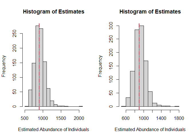
Figure 9: Left - histogram of estimates of abundance of clusters for systematic parallel design. Right - histogram of estimates of abundance of clusters for zigzag design.
par(oldparams)We can see in Figure 9 that there were a couple of high estimates generated >500 for both the parallel line and zigzag designs. These probably represent data sets that were difficult to fit a model too (perhaps a chance spiked data set). Most of the estimates are centered around truth but these occasional high estimates may have increased the mean value slightly and could be associated with the small amount of positive bias.
Simulation Conclusions
Under these simulation assumptions it appears that the zigzag design will cost us a little in accuracy but allow us to gain some precision. It should be noted that the cost in accuracy will vary depending on the distribution of animals in the survey region.