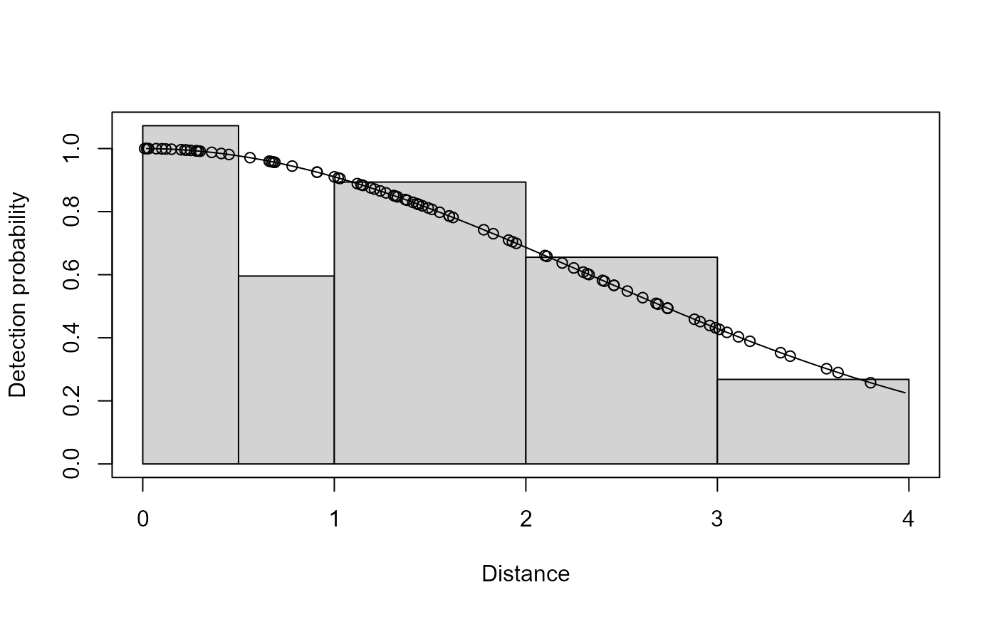
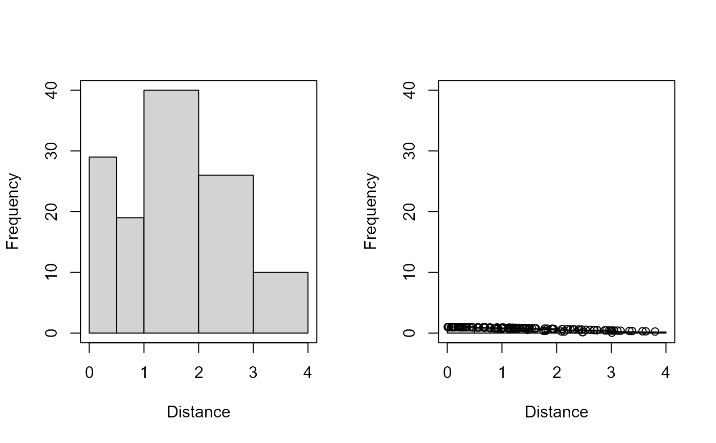
Plot fit of detection functions and histograms of data from distance sampling model

Plots the fitted detection function(s) with a histogram of the observed distances to compare visually the fitted model and data.

Usage

# S3 method for class 'ds'
plot(
  x,
  which = 2,
  breaks = NULL,
  nc = NULL,
  jitter.v = rep(0, 3),
  showpoints = TRUE,
  subset = NULL,
  pl.col = "lightgrey",
  pl.den = NULL,
  pl.ang = NULL,
  main = NULL,
  pages = 0,
  pdf = FALSE,
  ylim = NULL,
  xlab = "Distance",
  ylab = NULL,
  ...
)

Arguments

x

fitted model from ddf.

which

index to specify which plots should be produced:

1	histogram of observed distances
2	histogram of observed distances with fitted line and points (default)

breaks

user defined breakpoints

nc

number of equal width bins for histogram

jitter.v

apply jitter to points by multiplying the fitted value by a random draw from a normal distribution with mean 1 and sd jitter.v.

showpoints

logical variable; if TRUE plots predicted value for each observation (conditional on its observed distance).

subset

subset of data to plot.

pl.col

colour for histogram bars.

pl.den

shading density for histogram bars.

pl.ang

shading angle for histogram bars.

main

plot title.

pages

the number of pages over which to spread the plots. For example, if pages=1 then all plots will be displayed on one page. Default is 0, which prompts the user for the next plot to be displayed.

pdf

plot the histogram of distances with the PDF of the probability of detection overlaid. Ignored (with warning) for line transect models.

ylim

vertical axis limits.

xlab

horizontal axis label (defaults to "Distance").

ylab

vertical axis label (default automatically set depending on plot type).

...

other graphical parameters, passed to the plotting functions (plot, hist, lines, points, etc).

Value

Just plots.

Details

The structure of the histogram can be controlled by the user-defined arguments nc or breaks. The observation specific detection probabilities along with the line representing the fitted average detection probability.

It is not intended for the user to call plot.ds but its arguments are documented here. Instead the generic plot command should be used and it will call the appropriate function based on the class of the ddf object.

See also

add_df_covar_line

Author

Jeff Laake, Jon Bishop, David Borchers, David L Miller

Examples

# \donttest{
# fit a model to the tee data
data(book.tee.data)
egdata <- book.tee.data$book.tee.dataframe
xx <- ddf(dsmodel=~mcds(key="hn", formula=~sex),
          data=egdata[egdata$observer==1, ],
          method="ds", meta.data=list(width=4))

# not showing predicted probabilities
plot(xx, breaks=c(0, 0.5, 1, 2, 3, 4), showpoints=FALSE)


# two subsets
plot(xx, breaks=c(0, 0.5, 1, 2, 3, 4), subset=sex==0)

plot(xx, breaks=c(0, 0.5, 1, 2, 3, 4), subset=sex==1)


# put both plots on one page
plot(xx, breaks=c(0, 0.5, 1, 2, 3, 4), pages=1, which=1:2)

# }