Double platform analysis

Len Thomas

CREEM, Univ of St Andrews

November 2024

This example looks at mark-recapture distance sampling (MRDS) models. The first part of this exercise involves analysis of a survey of a known number of golf tees. This is intended mainly to familiarise you with the double-platform data structure and analysis features in the R function mrds (Laake, Borchers, Thomas, Miller, & Bishop, 2019).

To help understand the terminology using in MRDS and the output produced by mrds, there is a guide available at this link called Interpreting MRDS output: making sense of all the numbers.

Aims

The aims of this practical are to learn how to model

• trial and independent-observer configuration
• full and point independence assumptions,
• include covariates in the detection function(s) and
• select between competing models.

Golf tee data

These data come from a survey of golf tees which conducted by statistics students at the University of St Andrews. The data were collected along transect lines, 210 metres in total. A distance of 4 metres out from the centre line was searched and, for the purposes of this exercise, we assume that this comprised the total study area, which was divided into two strata. There were 250 clusters of tees in total and 760 individual tees in total.

The population was independently surveyed by two observer teams. The following data were recorded for each detected group: perpendicular distance, cluster size, observer (team 1 or 2), ‘sex’ (males are yellow and females are green and golf tees occur in single-sex clusters) and ‘exposure’. Exposure was a subjective judgment of whether the cluster was substantially obscured by grass (exposure=0) or not (exposure=1). The lengths of grass varied along the transect line and the grass was slightly more yellow along one part of the line compared to the rest.

The golf tee dataset is provided as part of the mrds package.

Open R and load the mrds package and golf tee dataset (called book.tee.data). The elements required for an MRDS analysis are contained within the object dataset. These data are in a hierarchical structure (rather than in a ‘flat file’ format) so that there are separate elements for observations, samples and regions. In the code below, each of these tables is extracted to avoid typing long names.

library(knitr)
library(mrds)
# Access the golf tee data
data(book.tee.data)
# Investigate the structure of the dataset
str(book.tee.data)

## List of 4
##  $ book.tee.dataframe:'data.frame':  324 obs. of  7 variables:
##   ..$ object  : num [1:324] 1 1 2 2 3 3 4 4 5 5 ...
##   ..$ observer: Factor w/ 2 levels "1","2": 1 2 1 2 1 2 1 2 1 2 ...
##   ..$ detected: num [1:324] 1 0 1 0 1 0 1 0 1 0 ...
##   ..$ distance: num [1:324] 2.68 2.68 3.33 3.33 0.34 0.34 2.53 2.53 1.46 1.46 ...
##   ..$ size    : num [1:324] 2 2 2 2 1 1 2 2 2 2 ...
##   ..$ sex     : num [1:324] 1 1 1 1 0 0 1 1 1 1 ...
##   ..$ exposure: num [1:324] 1 1 0 0 0 0 1 1 0 0 ...
##  $ book.tee.region   :'data.frame':  2 obs. of  2 variables:
##   ..$ Region.Label: Factor w/ 2 levels "1","2": 1 2
##   ..$ Area        : num [1:2] 1040 640
##  $ book.tee.samples  :'data.frame':  11 obs. of  3 variables:
##   ..$ Sample.Label: num [1:11] 1 2 3 4 5 6 7 8 9 10 ...
##   ..$ Region.Label: Factor w/ 2 levels "1","2": 1 1 1 1 1 1 2 2 2 2 ...
##   ..$ Effort      : num [1:11] 10 30 30 27 21 12 23 23 15 12 ...
##  $ book.tee.obs      :'data.frame':  162 obs. of  3 variables:
##   ..$ object      : int [1:162] 1 2 3 21 22 23 24 59 60 61 ...
##   ..$ Region.Label: int [1:162] 1 1 1 1 1 1 1 1 1 1 ...
##   ..$ Sample.Label: int [1:162] 1 1 1 1 1 1 1 1 1 1 ...

# Extract the list elements from the dataset into easy-to-access objects
detections <- book.tee.data$book.tee.dataframe # detection information
region <- book.tee.data$book.tee.region # region info
samples <- book.tee.data$book.tee.samples # transect info
obs <- book.tee.data$book.tee.obs # links detections to transects and regions

Examine the columns in the detections data because it has a particular structure.

# Check detections
head(detections)

##    object observer detected distance size sex exposure
## 1       1        1        1     2.68    2   1        1
## 21      1        2        0     2.68    2   1        1
## 2       2        1        1     3.33    2   1        0
## 22      2        2        0     3.33    2   1        0
## 3       3        1        1     0.34    1   0        0
## 23      3        2        0     0.34    1   0        0

The structure of the detection is as follows:

• each detected object (in this case the object was a group or cluster of golf tees) is given a unique number in the object column,
• each object occurs twice - once for observer 1 and once for observer 2,
• the detected column indicates whether the object was seen (detected=1) or not seen (detected=0) by the observer,
• perpendicular distance is in the distance column and cluster size is in the size column (the same default names as for the ds function).

To ensure that the variables sex and exposure are treated correctly, define them as factor variables.

# Define sex and exposure as factor variables 
detections$sex <- as.factor(detections$sex)
detections$exposure <- as.factor(detections$exposure)

Golf tee survey analyses

Estimation of p(0): distance only

We will start by analysing these data assuming that Observer 2 was generating trials for Observer 1 but not vice versa, i.e. trial configuration where Observer 1 is the primary and Observer 2 is the tracker. (The data could also be analysed in independent observer configuration - you are welcome to try this for yourself). We begin by assuming full independence (i.e. detections between observers are independent at all distances): this requires only a mark-recapture (MR) model and, to start with, perpendicular distance will be included as the only covariate.

# Fit trial configuration with full independence model
fi.mr.dist <- ddf(method='trial.fi', mrmodel=~glm(link='logit',formula=~distance),
                  data=detections, meta.data=list(width=4))

Examining mrds output

Having fitted the model, we can create tables summarizing the detection data. In the commands below, the tables are created using the det.tables function and saved to detection.tables.

# Create a set of tables summarizing the double observer data 
detection.tables <- det.tables(fi.mr.dist)
# Print these detection tables
print(detection.tables)

## 
## Observer 1 detections
##            Detected
##             Missed Detected
##   [0,0.4]        1       25
##   (0.4,0.8]      2       16
##   (0.8,1.2]      2       16
##   (1.2,1.6]      6       22
##   (1.6,2]        5        9
##   (2,2.4]        2       10
##   (2.4,2.8]      6       12
##   (2.8,3.2]      6        9
##   (3.2,3.6]      2        3
##   (3.6,4]        6        2
## 
## Observer 2 detections
##            Detected
##             Missed Detected
##   [0,0.4]        4       22
##   (0.4,0.8]      1       17
##   (0.8,1.2]      0       18
##   (1.2,1.6]      2       26
##   (1.6,2]        1       13
##   (2,2.4]        2       10
##   (2.4,2.8]      3       15
##   (2.8,3.2]      4       11
##   (3.2,3.6]      2        3
##   (3.6,4]        1        7
## 
## Duplicate detections
## 
##   [0,0.4] (0.4,0.8] (0.8,1.2] (1.2,1.6]   (1.6,2]   (2,2.4] (2.4,2.8] (2.8,3.2] 
##        21        15        16        20         8         8         9         5 
## (3.2,3.6]   (3.6,4] 
##         1         1 
## 
## Observer 1 detections of those seen by Observer 2
##           Missed Detected Prop. detected
## [0,0.4]        1       21      0.9545455
## (0.4,0.8]      2       15      0.8823529
## (0.8,1.2]      2       16      0.8888889
## (1.2,1.6]      6       20      0.7692308
## (1.6,2]        5        8      0.6153846
## (2,2.4]        2        8      0.8000000
## (2.4,2.8]      6        9      0.6000000
## (2.8,3.2]      6        5      0.4545455
## (3.2,3.6]      2        1      0.3333333
## (3.6,4]        6        1      0.1428571

The information in detection summary tables can be plotted, but, in the interest of space, only one (out of six possible plots) is shown (Figure 1).

# Plot detection information, change number to see other plots
plot(detection.tables, which=1)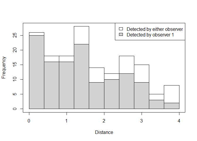

Figure 1: Detection distances for observer 1

The plot numbers are:

1. Histograms of distances for detections by either, or both, observers. The shaded regions show the number for observer 1.
2. Histograms of distances for detections by either, or both, observers. The shaded regions show the number for observer 2.
3. Histograms of distances for duplicates (detected by both observers).
4. Histogram of distances for detections by either, or both, observers. Not shown for trial configuration.
5. Histograms of distances for observer 2. The shaded regions indicate the number of duplicates - for example, the shaded region is the number of clusters in each distance bin that were detected by Observer 1 given that they were also detected by Observer 2 (the “|” symbol in the plot legend means “given that”).
6. Histograms of distances for observer 1. The shaded regions indicate the number of duplicates as for plot 5. Not shown for trial configuration.

Note that if an independent observer configuration had been chosen, all plots would be available.

A summary of the detection function model is available using the summary function. The Q-Q plot has the same interpretation as a Q-Q plot in a conventional, single platform analysis (Figure 2).

# Produce a summary of the fitted detection function object
summary(fi.mr.dist)

## 
## Summary for trial.fi object 
## Number of observations               :  162 
## Number seen by primary               :  124 
## Number seen by secondary (trials)    :  142 
## Number seen by both (detected trials):  104 
## AIC                                  :  452.8094 
## 
## 
## Conditional detection function parameters:
##              estimate        se
## (Intercept)  2.900233 0.4876238
## distance    -1.058677 0.2235722
## 
##                         Estimate          SE         CV
## Average p              0.6423252  0.04069410 0.06335435
## Average primary p(0)   0.9478579  0.06109656 0.06445750
## N in covered region  193.0486185 15.84826582 0.08209469

# Produce goodness of fit statistics and a qq plot
gof.result <- ddf.gof(fi.mr.dist, 
                      main="Full independence, trial configuration\ngoodness of fit Golf tee data")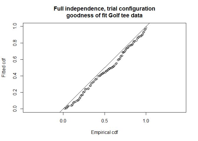

Figure 2: Fitted detection function for full independence, trial mode.

# Extract chi-square statistics for reporting
chi.distance <- gof.result$chisquare$chi1$chisq
chi.markrecap <- gof.result$chisquare$chi2$chisq
chi.total <- gof.result$chisquare$pooled.chi

Abbreviated \(\chi^2\) goodness-of-fit assessment shows the \(\chi^2\) contribution from the distance sampling model to be 11.5 and the \(\chi^2\) contribution from the mark-recapture model to be 3.4. The combination of these elements produces a total \(\chi^2\) of 14.9 with 17 degrees of freedom, resulting in a \(p\)-value of 0.604

The (two) detection functions can be plotted (Figure 3).

par(mfrow=c(1,2))
# Plot detection functions
plot(fi.mr.dist)

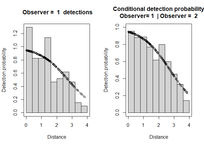
Figure 3: Observer 1 detection function (left) and conditional detection probabilty plot (right).

par(mfrow=c(1,1))

The plot labelled

• “Observer=1 detections” shows a histogram of Observer 1 detections with the estimated Observer 1 detection function overlaid on it and adjusted for p(0). The dots show the estimated detection probability for all Observer 1 detections.
• “Conditional detection probability” shows the proportion of Obs 2’s detections that were detected by Obs 1 (also see the detection tables). The fitted line is the estimated detection probability function for Obs 1 (given detection by Obs 2) - this is the MR model. Dots are estimated detection probabilities for each Obs 1 detection.

There is some evidence of unmodelled heterogeneity in that the fitted line in the left-hand plot declines more slowly than the histogram as the distance increases.

Estimating abundance

Abundance is estimated using the dht function. In this function, we need to supply information about the transects and survey regions.

# Calculate density estimates using the dht function
tee.abund <- dht(model=fi.mr.dist, region.table=region, sample.table=samples, obs.table=obs)
# Print out results in a nice format
knitr::kable(tee.abund$individuals$summary, digits=2, 
      caption="Survey summary statistics for golftees")

Table 1: Survey summary statistics for golftees

Region	Area	CoveredArea	Effort	n	k	ER	se.ER	cv.ER	mean.size	se.mean
1	1040	1040	130	229	6	1.76	0.12	0.07	3.18	0.21
2	640	640	80	152	5	1.90	0.33	0.18	2.92	0.23
Total	1680	1680	210	381	11	1.81	0.15	0.08	3.07	0.15

knitr::kable(tee.abund$individuals$N, digits=2, 
      caption="Abundance estimates for golftee population with two strata")

Table 1: Abundance estimates for golftee population with two strata

Label	Estimate	se	cv	lcl	ucl	df
1	356.52	32.35	0.09	294.54	431.53	17.13
2	236.64	44.14	0.19	147.33	380.09	5.06
Total	593.16	60.38	0.10	478.32	735.57	16.06

The estimated abundance is 593 (recall that the true abundance is 760) and so this estimate is negatively biased. The 95% confidence interval does not include the true value.

Estimation of p(0): distance and other explanatory variables

How about including the other covariates, size, sex and exposure, in the MR model? Which MR model would you use? In the command below, distance and sex are included in the detection function - remember sex was defined as a factor earlier on.

In the code below, all possible models (excluding interaction terms) are fitted.

# Full independence model
# Set up list with possible models
mr.formula <- c("~distance","~distance+size","~distance+sex","~distance+exposure",
                "~distance+size+sex","~distance+size+exposure","~distance+sex+exposure",
                "~distance+size+sex+exposure")
num.mr.models <- length(mr.formula)
# Create dataframe to store results
fi.results <- data.frame(MRmodel=mr.formula, AIC=rep(NA,num.mr.models))
# Loop through all MR models
for (i in 1:num.mr.models) {
  fi.model  <- ddf(method='trial.fi', 
                   mrmodel=~glm(link='logit',formula=as.formula(mr.formula[i])),
                  data=detections, meta.data=list(width=4))
  fi.results$AIC[i] <- summary(fi.model)$aic
}
# Calculate delta AIC
fi.results$deltaAIC <- fi.results$AIC - min(fi.results$AIC)
# Order by delta AIC
fi.results <- fi.results[order(fi.results$deltaAIC), ]
# Print results in pretty way
knitr::kable(fi.results, digits=2)

	MRmodel	AIC	deltaAIC
7	~distance+sex+exposure	405.68	0.00
8	~distance+size+sex+exposure	407.40	1.72
4	~distance+exposure	433.72	28.04
3	~distance+sex	434.41	28.74
6	~distance+size+exposure	435.33	29.65
5	~distance+size+sex	436.02	30.34
1	~distance	452.81	47.13
2	~distance+size	454.58	48.91

# Fit chosen model
fi.mr.dist.sex.exp  <- ddf(method='trial.fi', mrmodel=~glm(link='logit',formula=~distance+sex+exposure),
                           data=detections, meta.data=list(width=4))

We see that the preferred model contains distance + sex + exposure so check the goodness-of-fit statistics (Figure 4) and detection function plots (Figure 5).

# Check goodness-of-fit 
ddf.gof(fi.mr.dist.sex.exp, main="FI trial mode\nMR=dist+sex+exp")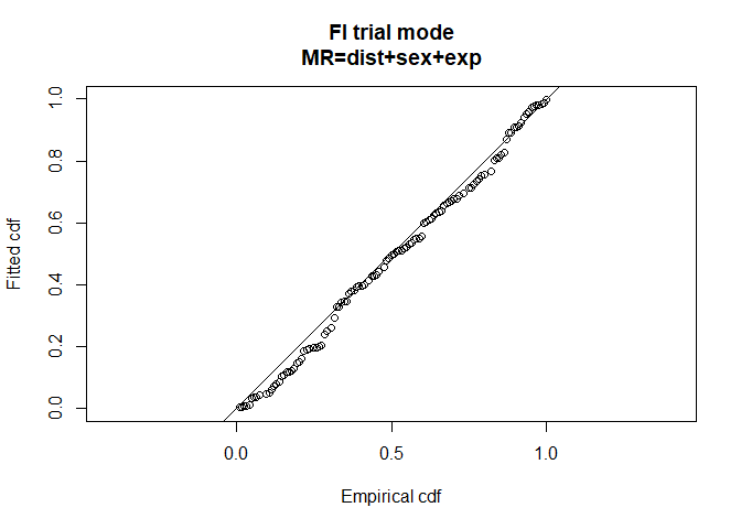

Figure 4: Preferred model goodness of fit.

## 
## Goodness of fit results for ddf object
## 
## Chi-square tests
## 
## Distance sampling component:
##           [0,0.4] (0.4,0.8] (0.8,1.2] (1.2,1.6] (1.6,2] (2,2.4] (2.4,2.8]
## Observed   25.000    16.000    16.000    22.000   9.000  10.000    12.000
## Expected   20.276    19.341    18.074    16.345  14.083  11.511     9.046
## Chisquare   1.101     0.577     0.238     1.957   1.834   0.198     0.964
##           (2.8,3.2] (3.2,3.6] (3.6,4]   Total
## Observed      9.000     3.000   2.000 124.000
## Expected      6.915     5.044   3.366 124.000
## Chisquare     0.629     0.828   0.554   8.881
## 
## No degrees of freedom for test
## 
## Mark-recapture component:
## Capture History 01
##           [0,0.4] (0.4,0.8] (0.8,1.2] (1.2,1.6] (1.6,2] (2,2.4] (2.4,2.8]
## Observed        1         2         2         6       5       2         6
## Expected        1         2         2         6       4       4         6
## Chisquare       0         0         0         0       0       1         0
##           (2.8,3.2] (3.2,3.6] (3.6,4] Total
## Observed          6         2       6    38
## Expected          7         2       5    38
## Chisquare         0         0       0     2
## Capture History 11
##           [0,0.4] (0.4,0.8] (0.8,1.2] (1.2,1.6] (1.6,2] (2,2.4] (2.4,2.8]
## Observed       21        15        16        20       8       8         9
## Expected       21        15        16        20       9       6         9
## Chisquare       0         0         0         0       0       1         0
##           (2.8,3.2] (3.2,3.6] (3.6,4] Total
## Observed          5         1       1   104
## Expected          4         1       2   104
## Chisquare         0         0       1     2
## 
## 
## Total chi-square = 12.205  P = 0.66344 with 15 degrees of freedom
## 
## Distance sampling Cramer-von Mises test (unweighted)
## Test statistic = 0.0976947 p-value = 0.596294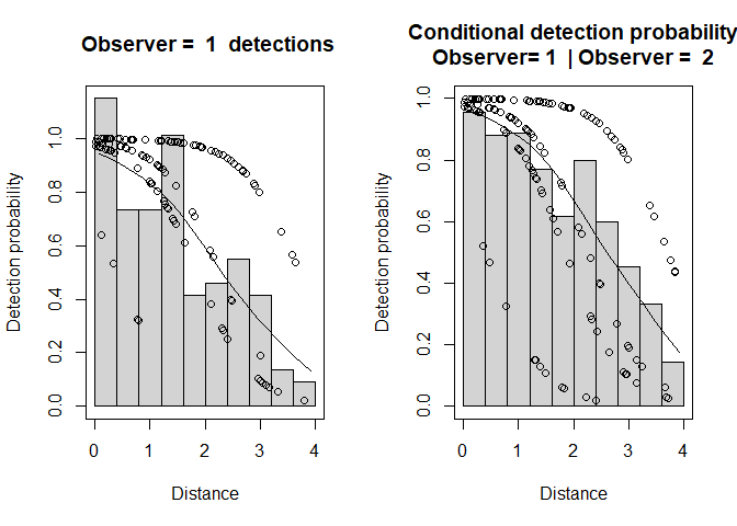

par(mfrow=c(1,2))
plot(fi.mr.dist.sex.exp)

Figure 5: Detection functions for full independence model with distance, sex and exposure in MR component.

And produce abundance estimates.

# Get abundance estimates 
tee.abund.fi <- dht(model=fi.mr.dist.sex.exp, region.table=region,
                    sample.table=samples, obs.table=obs)
# Print results
print(tee.abund.fi)

## Abundance and density estimates from distance sampling
## Variance       : R2, N/L 
## 
## Summary statistics
## 
##   Region Area CoveredArea Effort   n  k        ER      se.ER      cv.ER
## 1      1 1040        1040    130  72  6 0.5538462 0.02926903 0.05284685
## 2      2  640         640     80  52  5 0.6500000 0.08292740 0.12758061
## 3  Total 1680        1680    210 124 11 0.5904762 0.03641856 0.06167659
## 
## Summary for clusters
## 
## Abundance:
##   Region  Estimate       se        cv       lcl      ucl       df
## 1      1 119.28976 14.18666 0.1189260  91.64685 155.2704 10.12494
## 2      2  98.17731 18.59356 0.1893876  63.58200 151.5961  7.83844
## 3  Total 217.46707 26.05226 0.1197987 169.90391 278.3451 23.21368
## 
## Density:
##   Region  Estimate         se        cv        lcl       ucl       df
## 1      1 0.1147017 0.01364102 0.1189260 0.08812198 0.1492985 10.12494
## 2      2 0.1534020 0.02905244 0.1893876 0.09934687 0.2368689  7.83844
## 3  Total 0.1294447 0.01550730 0.1197987 0.10113328 0.1656816 23.21368
## 
## Summary for individuals
## 
## Abundance:
##   Region Estimate       se        cv      lcl      ucl        df
## 1      1 371.0397 37.86856 0.1020607 297.1733 463.2666 11.904084
## 2      2 279.7141 67.25221 0.2404320 154.4960 506.4208  5.482654
## 3  Total 650.7538 82.72649 0.1271241 493.7469 857.6875 11.907393
## 
## Density:
##   Region  Estimate         se        cv       lcl       ucl        df
## 1      1 0.3567690 0.03641208 0.1020607 0.2857436 0.4454487 11.904084
## 2      2 0.4370533 0.10508158 0.2404320 0.2414000 0.7912825  5.482654
## 3  Total 0.3873535 0.04924196 0.1271241 0.2938970 0.5105283 11.907393
## 
## Expected cluster size
##   Region Expected.S se.Expected.S cv.Expected.S
## 1      1   3.110407     0.2740170    0.08809682
## 2      2   2.849071     0.2211204    0.07761141
## 3  Total   2.992425     0.1758058    0.05875027

This model incorporates the effect of more variables causing the heterogeneity. The estimated abundance is 651 which is less biased than the previous estimate and the 95% confidence interval (494, 858) contains the true value.

The model is a reasonable fit to the data (i.e. non-significant \(\chi^2\) and Cramer von Mises tests). This model has a lower AIC (405.7) than the model with only distance (452.81) and so is to be preferred.

Point independence

A less restrictive assumption than full independence is point independence, which assumes that detections are only independent on the transect centre line i.e. at perpendicular distance zero (Buckland, Laake, & Borchers, 2010).

Determine if a simple point independence model is better than a simple full independence one. This requires that a distance sampling (DS) model is specified as well a MR model. Here we try a half-normal key function for the DS model (Figure 6).

# Fit trial configuration with point independence model
pi.mr.dist <- ddf(method='trial', 
                  mrmodel=~glm(link='logit', formula=~distance),
                  dsmodel=~cds(key='hn'), 
                  data=detections, meta.data=list(width=4))
# Summary pf the model 
summary(pi.mr.dist)

## 
## Summary for trial.fi object 
## Number of observations               :  162 
## Number seen by primary               :  124 
## Number seen by secondary (trials)    :  142 
## Number seen by both (detected trials):  104 
## AIC                                  :  140.8887 
## 
## 
## Conditional detection function parameters:
##              estimate        se
## (Intercept)  2.900233 0.4876238
## distance    -1.058677 0.2235722
## 
##                       Estimate         SE         CV
## Average primary p(0) 0.9478579 0.02409996 0.02542571
## 
## 
## 
## Summary for ds object
## Number of observations :  124 
## Distance range         :  0  -  4 
## AIC                    :  311.1385 
## Optimisation           :  mrds (nlminb) 
## 
## Detection function:
##  Half-normal key function 
## 
## Detection function parameters 
## Scale coefficient(s): 
##              estimate         se
## (Intercept) 0.6632435 0.09981249
## 
##            Estimate         SE         CV
## Average p 0.5842744 0.04637627 0.07937412
## 
## 
## Summary for trial object
## 
## Total AIC value =  452.0272 
##                        Estimate          SE         CV
## Average p             0.5538091  0.04615832 0.08334697
## N in covered region 223.9038534 22.99246338 0.10268900

# Produce goodness of fit statistics and a qq plot
gof.results <- ddf.gof(pi.mr.dist, 
                       main="Point independence, trial configuration\n goodness of fit Golftee data")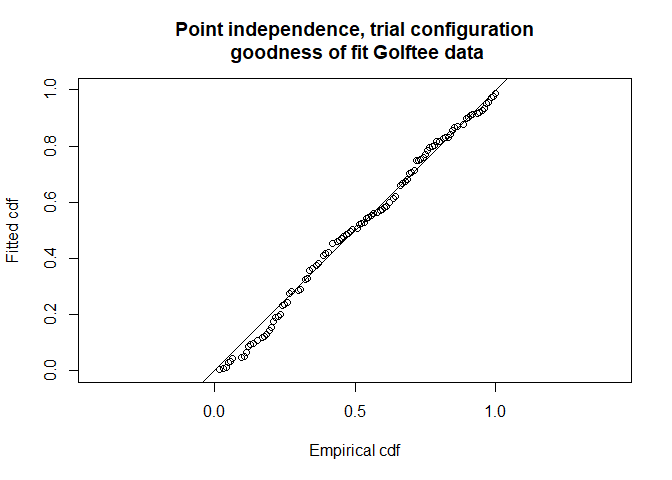

Figure 6: Point independence model in trial configuration goodness of fit.

The AIC for this point independence model is 452.03 which is marginally smaller than the first full independence model that was fitted and hence is to be preferred.

# Get abundance estimates 
tee.abund.pi <- dht(model=pi.mr.dist, region.table=region,
                    sample.table=samples, obs.table=obs)
# Print results
print(tee.abund.pi)

## Abundance and density estimates from distance sampling
## Variance       : R2, N/L 
## 
## Summary statistics
## 
##   Region Area CoveredArea Effort   n  k        ER      se.ER      cv.ER
## 1      1 1040        1040    130  72  6 0.5538462 0.02926903 0.05284685
## 2      2  640         640     80  52  5 0.6500000 0.08292740 0.12758061
## 3  Total 1680        1680    210 124 11 0.5904762 0.03641856 0.06167659
## 
## Summary for clusters
## 
## Abundance:
##   Region  Estimate       se         cv       lcl      ucl        df
## 1      1 130.00869 12.83042 0.09868894 106.66570 158.4601 48.427773
## 2      2  93.89516 14.30894 0.15239268  66.25307 133.0701  8.094137
## 3  Total 223.90385 23.21562 0.10368567 181.78333 275.7840 44.038262
## 
## Density:
##   Region  Estimate         se         cv       lcl       ucl        df
## 1      1 0.1250084 0.01233694 0.09868894 0.1025632 0.1523655 48.427773
## 2      2 0.1467112 0.02235771 0.15239268 0.1035204 0.2079220  8.094137
## 3  Total 0.1332761 0.01381882 0.10368567 0.1082044 0.1641571 44.038262
## 
## Summary for individuals
## 
## Abundance:
##   Region Estimate       se        cv      lcl      ucl        df
## 1      1 413.4999 44.00744 0.1064267 332.9536 513.5313 30.289360
## 2      2 274.4628 53.42626 0.1946576 171.1754 440.0740  5.987499
## 3  Total 687.9626 79.79844 0.1159924 542.4532 872.5040 25.993175
## 
## Density:
##   Region  Estimate         se        cv       lcl       ucl        df
## 1      1 0.3975960 0.04231485 0.1064267 0.3201477 0.4937801 30.289360
## 2      2 0.4288481 0.08347854 0.1946576 0.2674615 0.6876156  5.987499
## 3  Total 0.4095016 0.04749907 0.1159924 0.3228888 0.5193476 25.993175
## 
## Expected cluster size
##   Region Expected.S se.Expected.S cv.Expected.S
## 1      1   3.180556     0.2114629    0.06648615
## 2      2   2.923077     0.1750319    0.05987935
## 3  Total   3.072581     0.1391365    0.04528327

This results in an estimated abundance of 688. Can we do better if more covariates are included in the DS model?

Covariates in the DS model

To include covariates in the DS detection function, we need to specify an MCDS model as follows:

# Fit the PI-trial model - DS sex and MR distance 
pi.mr.dist.ds.sex <- ddf(method='trial', 
                         mrmodel=~glm(link='logit',formula=~distance),
                         dsmodel=~mcds(key='hn',formula=~sex), 
                         data=detections, meta.data=list(width=4))

Use the summary function to check the AIC and decide if you are going to include any additional covariates in the detection function.

Now try a point independence model that has the preferred MR model from your full independence analyses.

# Point independence model, Include covariates in DS model
# Use selected MR model, iterate across DS models
ds.formula <- c("~size","~sex","~exposure","~size+sex","~size+exposure","~sex+exposure",
                "~size+sex+exposure")
num.ds.models <- length(ds.formula)
# Create dataframe to store results
pi.results <- data.frame(DSmodel=ds.formula, AIC=rep(NA,num.ds.models))
# Loop through ds models - use selected MR model from earlier
for (i in 1:num.ds.models) {
  pi.model <- ddf(method='trial', mrmodel=~glm(link='logit',formula=~distance+sex+exposure),
                  dsmodel=~mcds(key='hn',formula=as.formula(ds.formula[i])), 
                  data=detections, meta.data=list(width=4))
  pi.results$AIC[i] <- summary(pi.model)$AIC
}
# Calculate delta AIC
pi.results$deltaAIC <- pi.results$AIC - min(pi.results$AIC)
# Order by delta AIC
pi.results <- pi.results[order(pi.results$deltaAIC), ]
knitr::kable(pi.results, digits = 2)

	DSmodel	AIC	deltaAIC
2	~sex	399.26	0.00
6	~sex+exposure	400.28	1.02
4	~size+sex	401.06	1.80
7	~size+sex+exposure	401.94	2.69
1	~size	407.92	8.66
3	~exposure	407.97	8.72
5	~size+exposure	409.89	10.63

This indicates that sex should be included in the DS model. We do this and check the goodness of fit and obtain abundance (Figure 7).

# Fit chosen model
pi.ds.sex <- ddf(method='trial', mrmodel=~glm(link='logit',formula=~distance+sex+exposure),
                dsmodel=~mcds(key='hn',formula=~sex), data=detections,  
                meta.data=list(width=4))
summary(pi.ds.sex)

## 
## Summary for trial.fi object 
## Number of observations               :  162 
## Number seen by primary               :  124 
## Number seen by secondary (trials)    :  142 
## Number seen by both (detected trials):  104 
## AIC                                  :  94.89911 
## 
## 
## Conditional detection function parameters:
##               estimate        se
## (Intercept)  0.7870962 0.6774633
## distance    -1.9435496 0.3706866
## sex1         2.8059863 0.6828331
## exposure1    3.6094527 0.7332797
## 
##                       Estimate         SE         CV
## Average primary p(0) 0.9697357 0.02018875 0.02081882
## 
## 
## 
## Summary for ds object
## Number of observations :  124 
## Distance range         :  0  -  4 
## AIC                    :  304.3594 
## Optimisation           :  mrds (nlminb) 
## 
## Detection function:
##  Half-normal key function 
## 
## Detection function parameters 
## Scale coefficient(s): 
##              estimate        se
## (Intercept) 0.2525377 0.1327279
## sex1        0.5832341 0.2041094
## 
##            Estimate         SE        CV
## Average p 0.5605421 0.04616356 0.0823552
## 
## 
## Summary for trial object
## 
## Total AIC value =  399.2585 
##                        Estimate          SE         CV
## Average p             0.5435777  0.04643912 0.08543235
## N in covered region 228.1182656 24.21303261 0.10614245

# Check goodness-of-fit 
ddf.gof(pi.ds.sex, main="PI trial configutation\nGolfTee DS model sex")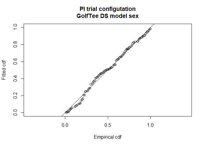

Figure 7: Goodness of fit of point independence model with sex covariate in the distance sampling component and distance, sex and exposure in the mr component.

## 
## Goodness of fit results for ddf object
## 
## Chi-square tests
## 
## Distance sampling component:
##           [0,0.4] (0.4,0.8] (0.8,1.2] (1.2,1.6] (1.6,2] (2,2.4] (2.4,2.8]
## Observed   25.000    16.000    16.000    22.000   9.000  10.000    12.000
## Expected   21.917    20.740    18.630    15.976  13.181  10.553     8.261
## Chisquare   0.434     1.083     0.371     2.272   1.326   0.029     1.692
##           (2.8,3.2] (3.2,3.6] (3.6,4]   Total
## Observed      9.000     3.000   2.000 124.000
## Expected      6.354     4.810   3.579 124.000
## Chisquare     1.102     0.681   0.697   9.687
## 
## P = 0.20699 with 7 degrees of freedom
## 
## Mark-recapture component:
## Capture History 01
##           [0,0.4] (0.4,0.8] (0.8,1.2] (1.2,1.6] (1.6,2] (2,2.4] (2.4,2.8]
## Observed        1         2         2         6       5       2         6
## Expected        1         2         2         6       4       4         6
## Chisquare       0         0         0         0       0       1         0
##           (2.8,3.2] (3.2,3.6] (3.6,4] Total
## Observed          6         2       6    38
## Expected          7         2       5    38
## Chisquare         0         0       0     2
## Capture History 11
##           [0,0.4] (0.4,0.8] (0.8,1.2] (1.2,1.6] (1.6,2] (2,2.4] (2.4,2.8]
## Observed       21        15        16        20       8       8         9
## Expected       21        15        16        20       9       6         9
## Chisquare       0         0         0         0       0       1         0
##           (2.8,3.2] (3.2,3.6] (3.6,4] Total
## Observed          5         1       1   104
## Expected          4         1       2   104
## Chisquare         0         0       1     2
## 
## MR total chi-square = 3.3242  P = 0.76719 with 6 degrees of freedom
## 
## 
## Total chi-square = 13.012  P = 0.44692 with 13 degrees of freedom
## 
## Distance sampling Cramer-von Mises test (unweighted)
## Test statistic = 0.081285 p-value = 0.684457

# Get abundance estimates 
tee.abund.pi.ds.sex <- dht(model=pi.ds.sex, region.table=region,
                    sample.table=samples, obs.table=obs)
print(tee.abund.pi.ds.sex)

## Abundance and density estimates from distance sampling
## Variance       : R2, N/L 
## 
## Summary statistics
## 
##   Region Area CoveredArea Effort   n  k        ER      se.ER      cv.ER
## 1      1 1040        1040    130  72  6 0.5538462 0.02926903 0.05284685
## 2      2  640         640     80  52  5 0.6500000 0.08292740 0.12758061
## 3  Total 1680        1680    210 124 11 0.5904762 0.03641856 0.06167659
## 
## Summary for clusters
## 
## Abundance:
##   Region Estimate       se        cv       lcl      ucl        df
## 1      1 125.7678 12.50301 0.0994134 102.97968 153.5987 43.661605
## 2      2 102.3504 17.53164 0.1712904  68.75816 152.3544  7.394232
## 3  Total 228.1183 25.15313 0.1102635 182.12587 285.7252 28.045408
## 
## Density:
##   Region  Estimate         se        cv        lcl       ucl        df
## 1      1 0.1209306 0.01202212 0.0994134 0.09901892 0.1476911 43.661605
## 2      2 0.1599226 0.02739319 0.1712904 0.10743463 0.2380538  7.394232
## 3  Total 0.1357847 0.01497210 0.1102635 0.10840826 0.1700745 28.045408
## 
## Summary for individuals
## 
## Abundance:
##   Region Estimate       se         cv      lcl      ucl        df
## 1      1 395.0545 36.33887 0.09198445 329.0893 474.2422 79.293122
## 2      2 299.7763 65.43246 0.21827099 175.5600 511.8809  5.685162
## 3  Total 694.8307 84.25522 0.12126006 537.2149 898.6902 15.167148
## 
## Density:
##   Region  Estimate         se         cv       lcl       ucl        df
## 1      1 0.3798601 0.03494122 0.09198445 0.3164320 0.4560021 79.293122
## 2      2 0.4684004 0.10223822 0.21827099 0.2743125 0.7998140  5.685162
## 3  Total 0.4135897 0.05015192 0.12126006 0.3197708 0.5349347 15.167148
## 
## Expected cluster size
##   Region Expected.S se.Expected.S cv.Expected.S
## 1      1   3.141141     0.2081675    0.06627129
## 2      2   2.928920     0.1866200    0.06371632
## 3  Total   3.045923     0.1371508    0.04502767

This model estimated an abundance of 695, which is closest to the true value of all the models - it is still less than the true value indicating, perhaps, some unmodelled heterogeneity on the trackline (or perhaps just bad luck - remember this was only one survey).

Was this complex modelling worthwhile? In this case, the estimated \(p(0)\) for the best model was 0.97 (which is very close to 1). If we ran a conventional distance sampling analysis, pooling the data from the two observers, we should get a very robust estimate of true abundance.

References

Buckland, S. T., Laake, J. L., & Borchers, D. L. (2010). Double-observer line transect methods: Levels of independence. Biometrics, 66, 169–177. https://doi.org/10.1111/j.1541-0420.2009.01239.x

Laake, J., Borchers, D., Thomas, L., Miller, D., & Bishop, J. (2019). Mrds: Mark-recapture distance sampling.