Multiple surveys by different observers of a single 1km transect containing 150 wooden stakes placed randomly throughout a 40 m strip (20m on either side).
Format
A data frame with 150 observations on the following 10 variables.
- StakeNo
unique number for each stake 1-150
- PD
perpendicular distance at which the stake was placed from the line
- Obs1
0/1 whether missed/seen by observer 1
- Obs2
0/1 whether missed/seen by observer 2
- Obs3
0/1 whether missed/seen by observer 3
- Obs4
0/1 whether missed/seen by observer 4
- Obs5
0/1 whether missed/seen by observer 5
- Obs6
0/1 whether missed/seen by observer 6
- Obs7
0/1 whether missed/seen by observer 7
- Obs8
0/1 whether missed/seen by observer 8
Source
Laake, J. 1978. Line transect estimators robust to animal movement. M.S. Thesis. Utah State University, Logan, Utah. 55p.
References
Burnham, K. P., D. R. Anderson, and J. L. Laake. 1980. Estimation of Density from Line Transect Sampling of Biological Populations. Wildlife Monographs:7-202.
Examples
# \donttest{
data(stake77)
# Extract functions for stake data and put in the mrds format
extract.stake <- function(stake,obs){
extract.obs <- function(obs){
example <- subset(stake,eval(parse(text=paste("Obs",obs,"==1",sep=""))),
select="PD")
example$distance <- example$PD
example$object <- 1:nrow(example)
example$PD <- NULL
return(example)
}
if(obs!="all"){
return(extract.obs(obs=obs))
}else{
example <- NULL
for(i in 1:(ncol(stake)-2)){
df <- extract.obs(obs=i)
df$person <- i
example <- rbind(example,df)
}
example$person <- factor(example$person)
example$object <- 1:nrow(example)
return(example)
}
}
extract.stake.pairs <- function(stake,obs1,obs2,removal=FALSE){
obs1 <- paste("Obs",obs1,sep="")
obs2 <- paste("Obs",obs2,sep="")
example <- subset(stake,eval(parse(text=paste(obs1,"==1 |",obs2,"==1 ",
sep=""))),select=c("PD",obs1,obs2))
names(example) <- c("distance","obs1","obs2")
detected <- c(example$obs1,example$obs2)
example <- data.frame(object = rep(1:nrow(example),2),
distance = rep(example$distance,2),
detected = detected,
observer = c(rep(1,nrow(example)),
rep(2,nrow(example))))
if(removal) example$detected[example$observer==2] <- 1
return(example)
}
# extract data for observer 1 and fit a single observer model
stakes <- extract.stake(stake77,1)
ds.model <- ddf(dsmodel = ~mcds(key = "hn", formula = ~1), data = stakes,
method = "ds", meta.data = list(width = 20))
plot(ds.model,breaks=seq(0,20,2),showpoints=TRUE)
 ddf.gof(ds.model)
 #>
#> Goodness of fit results for ddf object
#>
#> Chi-square tests
#> [0,2.22] (2.22,4.44] (4.44,6.67] (6.67,8.89] (8.89,11.1] (11.1,13.3]
#> Observed 13.000 17.000 14.000 12.000 11.000 5.000
#> Expected 16.023 15.107 13.430 11.256 8.894 6.627
#> Chisquare 0.570 0.237 0.024 0.049 0.498 0.399
#> (13.3,15.6] (15.6,17.8] (17.8,20] Total
#> Observed 3.000 3.000 3.000 81.00
#> Expected 4.655 3.083 1.925 81.00
#> Chisquare 0.588 0.002 0.600 2.97
#>
#> P = 0.8878 with 7 degrees of freedom
#>
#> Distance sampling Cramer-von Mises test (unweighted)
#> Test statistic = 0.051489 p-value = 0.867184
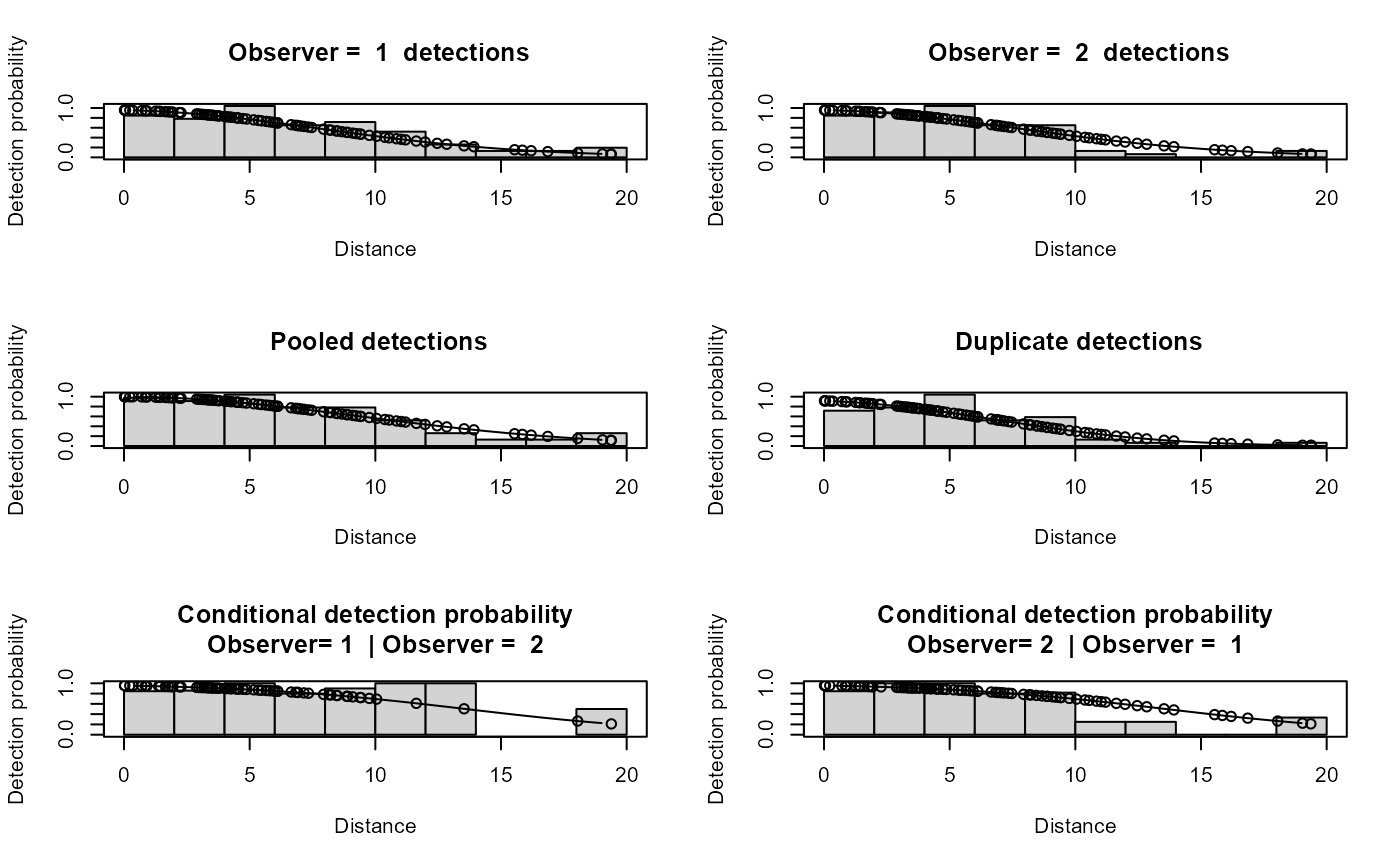
# extract data from observers 1 and 3 and fit an io model
stkpairs <- extract.stake.pairs(stake77,1,3,removal=FALSE)
io.model <- ddf(dsmodel = ~mcds(key = "hn", formula=~1),
mrmodel=~glm(formula=~distance),
data = stkpairs, method = "io")
#> Warning: no truncation distance specified; using largest observed distance
summary(io.model)
#>
#> Summary for io.fi object
#> Number of observations : 89
#> Number seen by primary : 81
#> Number seen by secondary : 68
#> Number seen by both : 60
#> AIC : 137.046
#>
#>
#> Conditional detection function parameters:
#> estimate se
#> (Intercept) 3.105418 0.52079895
#> distance -0.228405 0.05957038
#>
#> Estimate SE CV
#> Average primary p(0) 0.9571157 0.021376325 0.022334108
#> Average secondary p(0) 0.9571157 0.021376325 0.022334108
#> Average combined p(0) 0.9981609 0.001833418 0.001836796
#>
#>
#> Summary for ds object
#> Number of observations : 89
#> Distance range : 0 - 19.39
#> AIC : 504.1853
#> Optimisation : mrds (nlminb)
#>
#> Detection function:
#> Half-normal key function
#>
#> Detection function parameters
#> Scale coefficient(s):
#> estimate se
#> (Intercept) 2.233369 0.1031155
#>
#> Estimate SE CV
#> Average p 0.5803993 0.04794403 0.08260525
#>
#>
#> Summary for io object
#> Total AIC value : 641.2313
#>
#> Estimate SE CV
#> Average p 0.5793319 0.04786769 0.08262567
#> N in covered region 153.6252334 16.51282572 0.10748772
par(mfrow=c(3,2))
plot(io.model,breaks=seq(0,20,2),showpoints=TRUE,new=FALSE)
#>
#> Goodness of fit results for ddf object
#>
#> Chi-square tests
#> [0,2.22] (2.22,4.44] (4.44,6.67] (6.67,8.89] (8.89,11.1] (11.1,13.3]
#> Observed 13.000 17.000 14.000 12.000 11.000 5.000
#> Expected 16.023 15.107 13.430 11.256 8.894 6.627
#> Chisquare 0.570 0.237 0.024 0.049 0.498 0.399
#> (13.3,15.6] (15.6,17.8] (17.8,20] Total
#> Observed 3.000 3.000 3.000 81.00
#> Expected 4.655 3.083 1.925 81.00
#> Chisquare 0.588 0.002 0.600 2.97
#>
#> P = 0.8878 with 7 degrees of freedom
#>
#> Distance sampling Cramer-von Mises test (unweighted)
#> Test statistic = 0.051489 p-value = 0.867184
# extract data from observers 1 and 3 and fit an io model
stkpairs <- extract.stake.pairs(stake77,1,3,removal=FALSE)
io.model <- ddf(dsmodel = ~mcds(key = "hn", formula=~1),
mrmodel=~glm(formula=~distance),
data = stkpairs, method = "io")
#> Warning: no truncation distance specified; using largest observed distance
summary(io.model)
#>
#> Summary for io.fi object
#> Number of observations : 89
#> Number seen by primary : 81
#> Number seen by secondary : 68
#> Number seen by both : 60
#> AIC : 137.046
#>
#>
#> Conditional detection function parameters:
#> estimate se
#> (Intercept) 3.105418 0.52079895
#> distance -0.228405 0.05957038
#>
#> Estimate SE CV
#> Average primary p(0) 0.9571157 0.021376325 0.022334108
#> Average secondary p(0) 0.9571157 0.021376325 0.022334108
#> Average combined p(0) 0.9981609 0.001833418 0.001836796
#>
#>
#> Summary for ds object
#> Number of observations : 89
#> Distance range : 0 - 19.39
#> AIC : 504.1853
#> Optimisation : mrds (nlminb)
#>
#> Detection function:
#> Half-normal key function
#>
#> Detection function parameters
#> Scale coefficient(s):
#> estimate se
#> (Intercept) 2.233369 0.1031155
#>
#> Estimate SE CV
#> Average p 0.5803993 0.04794403 0.08260525
#>
#>
#> Summary for io object
#> Total AIC value : 641.2313
#>
#> Estimate SE CV
#> Average p 0.5793319 0.04786769 0.08262567
#> N in covered region 153.6252334 16.51282572 0.10748772
par(mfrow=c(3,2))
plot(io.model,breaks=seq(0,20,2),showpoints=TRUE,new=FALSE)
 dev.new()
ddf.gof(io.model)
#>
#> Goodness of fit results for ddf object
#>
#> Chi-square tests
#>
#> Distance sampling component:
#> [0,2.42] (2.42,4.85] (4.85,7.27] (7.27,9.7] (9.7,12.1] (12.1,14.5]
#> Observed 17.000 21.000 16.000 14.000 9.000 4.000
#> Expected 18.954 17.725 15.499 12.673 9.690 6.929
#> Chisquare 0.202 0.605 0.016 0.139 0.049 1.238
#> (14.5,17] (17,19.4] Total
#> Observed 4.000 4.000 89.000
#> Expected 4.633 2.897 89.000
#> Chisquare 0.086 0.420 2.756
#>
#> P = 0.8388 with 6 degrees of freedom
#>
#> Mark-recapture component:
#> Capture History 10
#> [0,2.42] (2.42,4.85] (4.85,7.27] (7.27,9.7] (9.7,12.1] (12.1,14.5]
#> Observed 2 0 1 3 6 3
#> Expected 1 2 2 3 2 1
#> Chisquare 1 2 1 0 6 2
#> (14.5,17] (17,19.4] Total
#> Observed 4 2 21
#> Expected 2 2 14
#> Chisquare 4 0 16
#> Capture History 01
#> [0,2.42] (2.42,4.85] (4.85,7.27] (7.27,9.7] (9.7,12.1] (12.1,14.5]
#> Observed 3 1 2 1 0 0
#> Expected 1 2 2 3 2 1
#> Chisquare 5 0 0 1 2 1
#> (14.5,17] (17,19.4] Total
#> Observed 0 1 8
#> Expected 2 2 14
#> Chisquare 2 0 12
#> Capture History 11
#> [0,2.42] (2.42,4.85] (4.85,7.27] (7.27,9.7] (9.7,12.1] (12.1,14.5]
#> Observed 12 20 13 10 3 1
#> Expected 15 17 12 9 4 1
#> Chisquare 1 0 0 0 0 0
#> (14.5,17] (17,19.4] Total
#> Observed 0 1 60
#> Expected 1 1 60
#> Chisquare 1 0 3
#>
#> MR total chi-square = 31.176 P = 0.0052374 with 14 degrees of freedom
#>
#>
#> Total chi-square = 33.932 P = 0.026589 with 20 degrees of freedom
#>
#> Distance sampling Cramer-von Mises test (unweighted)
#> Test statistic = 0.0468697 p-value = 0.895003
# }
dev.new()
ddf.gof(io.model)
#>
#> Goodness of fit results for ddf object
#>
#> Chi-square tests
#>
#> Distance sampling component:
#> [0,2.42] (2.42,4.85] (4.85,7.27] (7.27,9.7] (9.7,12.1] (12.1,14.5]
#> Observed 17.000 21.000 16.000 14.000 9.000 4.000
#> Expected 18.954 17.725 15.499 12.673 9.690 6.929
#> Chisquare 0.202 0.605 0.016 0.139 0.049 1.238
#> (14.5,17] (17,19.4] Total
#> Observed 4.000 4.000 89.000
#> Expected 4.633 2.897 89.000
#> Chisquare 0.086 0.420 2.756
#>
#> P = 0.8388 with 6 degrees of freedom
#>
#> Mark-recapture component:
#> Capture History 10
#> [0,2.42] (2.42,4.85] (4.85,7.27] (7.27,9.7] (9.7,12.1] (12.1,14.5]
#> Observed 2 0 1 3 6 3
#> Expected 1 2 2 3 2 1
#> Chisquare 1 2 1 0 6 2
#> (14.5,17] (17,19.4] Total
#> Observed 4 2 21
#> Expected 2 2 14
#> Chisquare 4 0 16
#> Capture History 01
#> [0,2.42] (2.42,4.85] (4.85,7.27] (7.27,9.7] (9.7,12.1] (12.1,14.5]
#> Observed 3 1 2 1 0 0
#> Expected 1 2 2 3 2 1
#> Chisquare 5 0 0 1 2 1
#> (14.5,17] (17,19.4] Total
#> Observed 0 1 8
#> Expected 2 2 14
#> Chisquare 2 0 12
#> Capture History 11
#> [0,2.42] (2.42,4.85] (4.85,7.27] (7.27,9.7] (9.7,12.1] (12.1,14.5]
#> Observed 12 20 13 10 3 1
#> Expected 15 17 12 9 4 1
#> Chisquare 1 0 0 0 0 0
#> (14.5,17] (17,19.4] Total
#> Observed 0 1 60
#> Expected 1 1 60
#> Chisquare 1 0 3
#>
#> MR total chi-square = 31.176 P = 0.0052374 with 14 degrees of freedom
#>
#>
#> Total chi-square = 33.932 P = 0.026589 with 20 degrees of freedom
#>
#> Distance sampling Cramer-von Mises test (unweighted)
#> Test statistic = 0.0468697 p-value = 0.895003
# }