Getting Started with dssd
L. Marshall
CREEM, Univ of St AndrewsSeptember 2025
Source:vignettes/GettingStarted.Rmd
GettingStarted.RmdSurvey Design for Distance Sampling
The most up-to-date copies of these vignettes can now be found on the distance sampling examples page of our website: https://distancesampling.org/resources/vignettes.html
Distance Sampling techniques provide design based estimates of density and abundance for populations, the accuracy of these estimates therefore relies on valid survey design. The process of designing a survey involves deciding on the required survey effort in order to achieve a desired precision followed by deciding where exactly the effort (the lines or points) will be located within the survey region.
Before proceeding to the design stage there are a number of considerations which first need to be addressed. The first steps in conducting a survey are to clearly define the study population and the objectives of the study. In addition, the use of spatial stratification to improve precision should also be considered, the ‘Multiple Strata in dssd’ vignette details how to work with multi-strata study regions. We recommend consulting Buckland et al. (2001) chapter 7 and Strindberg, Buckland, and Thomas (2004) before using dssd to design your distance sampling survey.
Once you have defined your population and study objectives, and estimated the required effort, dssd (Marshall 2019a) can help ensure you meet the survey design assumptions associated with distance sampling. Distance sampling assumes that the survey transects are a representative sample of the study region and are laid out at random with respect to the population. dssd achieves both these objectives by randomising the locations of the transects. Designs may be fully random with each transect being randomly located independently of other transects or a systematic design with a random start point should also meet this assumption.
The next assumption is that each point within the study region is equally likely to be sampled as any other, we call this uniform coverage. We can assess the coverage across the study region using a grid of points called a coverage grid. Some designs have more uniform coverage than others and dssd can help assess how uniform the coverage is via simulation. If non-uniform coverage is of concern dssd can be used in conjunction with DSsim (Marshall 2019b) the distance sampling simulations package to better assess the effects of non-uniform coverage under normal and worst case scenarios to allow a more informed choice of design.
Setting up the Region
The first step in creating a survey design is to set up your study region. The easiest way to do this is using a shapefile which has already been created to define your study region. The dssd package contains the example shapefile used in this vignette and can be accessed using the code below. Here we use this shapefile to define the study region and then plot it.
library(dssd)
shapefile.name <- system.file("extdata", "TrackExample.shp", package = "dssd")
region <- make.region(region.name = "study area",
                      shape = shapefile.name)
plot(region)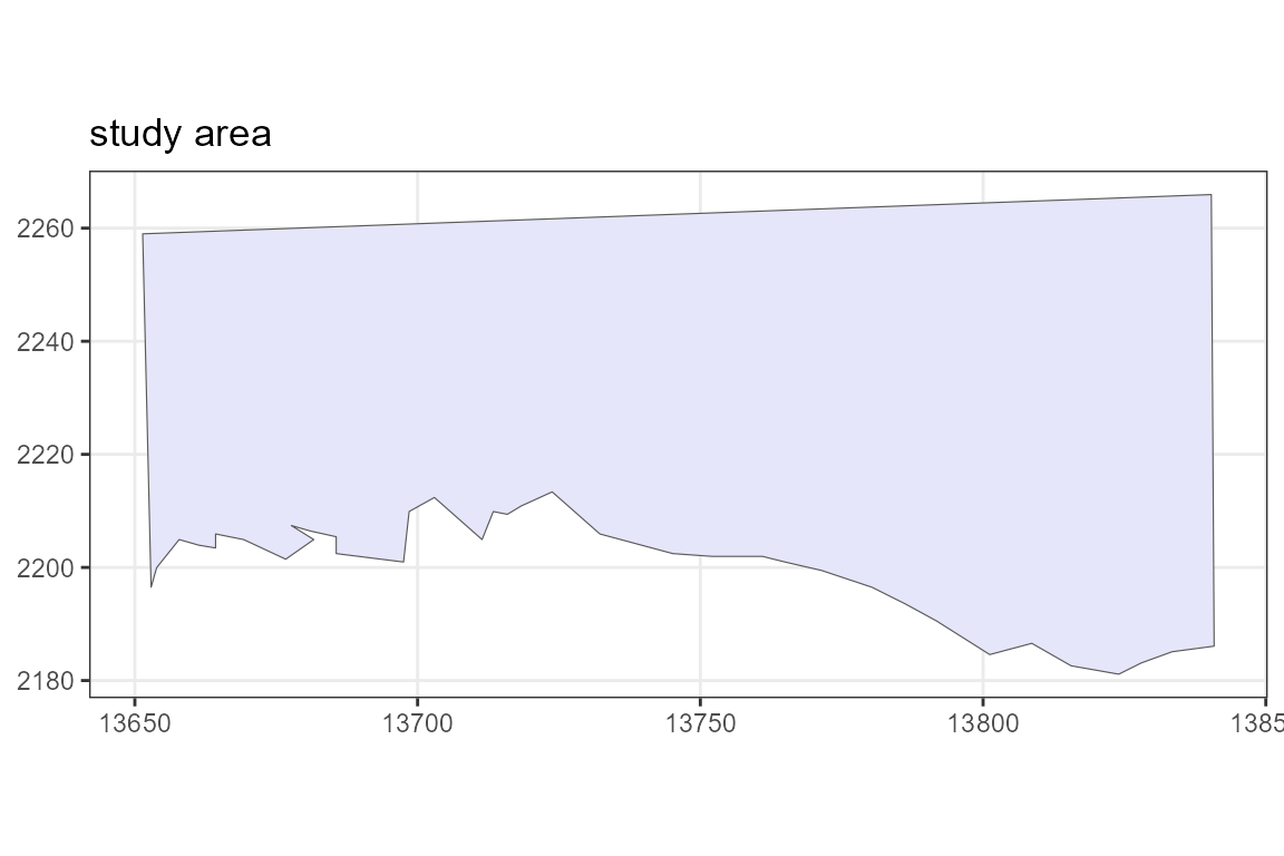
Figure 1: The study region.
Creating a Coverage Grid
Ideally, a coverage grid is created separately before creating the design. The same coverage grid can then be used for multiple designs. If a coverage grid is not passed to the design then this will be detected when the coverage simulation is run and a grid with 1000 points will automatically be generated.
cover <- make.coverage(region,
                       n.grid.points = 1000)
Defining the Design
dssd provides a number of point and line transect designs. The design refers to a description of how the transect locations are selected and does not specify the locations of a single set of transects. We will later refer to a single set of transects generated from the design as a survey. A survey can then be thought if as a single random realisation of a design.
Here we will demonstrate a systematic parallel line design. We will define the desired effort as 1300 km. Note that the line length units will always be the same as the region coordinate units. Usually edge effects for line transect surveys are minimal so we will choose to carry out minus sampling, when only transects within the survey region are sampled. The design angle for parallel line designs is 0 for vertical lines and then moves round in a clockwise direction. Here I have left the design angle as 0 as this maximises the number of transects, the study region is larger in the x-dimension than the y-dimension. I have set the truncation distance to be 2 km, this is the maximum distance at which it is possible to make detections and is used to define the covered area. The covered area refers to the area of the study region which is sampled during the survey, this is a set of rectangles around line transects or a set of circles around point transects which are then clipped to the strata boundaries. If these rectangles or circles overlap, then the areas of overlap are counted twice. This means that it is possible, with a sufficiently large truncation distance, to sample more than 100% of the survey region.
design <- make.design(region = region,
                      design = "systematic",
                      line.length = 1300,
                      edge.protocol = "minus",
                      design.angle = 0,
                      truncation = 2,
                      coverage.grid = cover)
Generating a Survey
Now we have defined the design we should check that it generated transects as we would expect by generating a survey. You can then view statistics about this survey and plot the transects.
transects <- generate.transects(design)
transects
##
## Strata study area:
## ___________________
## Design: systematically spaced parallel transects
## Spacing: 9.258935
## Line length: 1346.139
## Trackline length: 1536.667
## Cyclic trackline length: 1722.431
## Number of samplers: 21
## Design angle: 0
## Edge protocol: minus
## Covered area: 5282.704
## Strata coverage: 43.89%
## Strata area: 12036.62
##
## Study Area Totals:
## _________________
## Line length: 1346.139
## Trackline length: 1536.667
## Cyclic trackline length: 1722.431
## Number of samplers: 21
## Covered area: 5282.704
## Average coverage: 43.89%
plot(region, transects)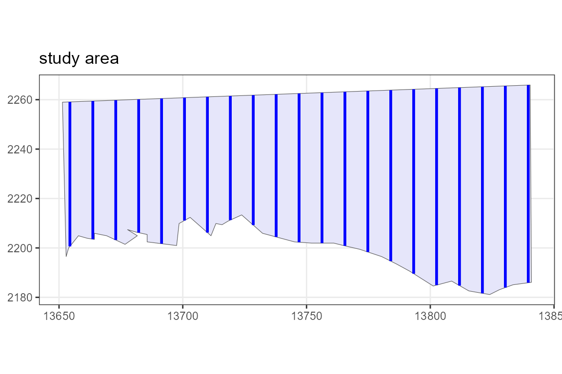
Figure 2: An example set of transects generated from the design plotted within the study region.
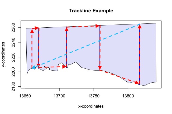
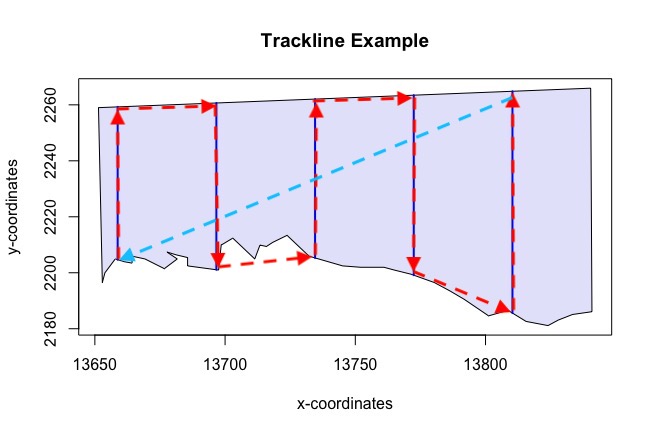
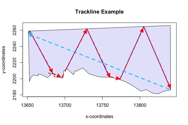
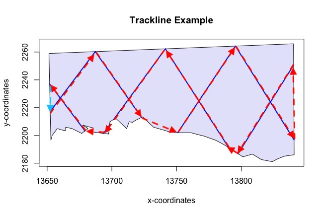
We can see that this survey has an on effort line length of 1346 km, close to the 1300 km we asked for. It was generated based on a spacing of 9.26 km, a value calculated based on the requested line length, and resulted in 21 transects. We are also given the trackline length and cyclic trackline lengths. The trackline length is the sum of the lengths of the transects plus the off-effort transit time required to complete the survey from the beginning of the first transect to the end of the last transect. The off-effort transit distance is calculated as the crow flies and may be longer in reality if transit is required around lakes, islands or coastlines etc. The cyclic trackline length is the trackline length plus the off-effort transit distance required to return from the end of the last transect to the beginning of the first transect. Please see the appendix for more details and figures.
We are also told that this survey covers 43.9% of the study area. If we wish to view the covered area for this particular set of transects we can plot it using the code below. The covered area is the rectangles delineated by the black lines.
plot(region, transects, covered.area = TRUE)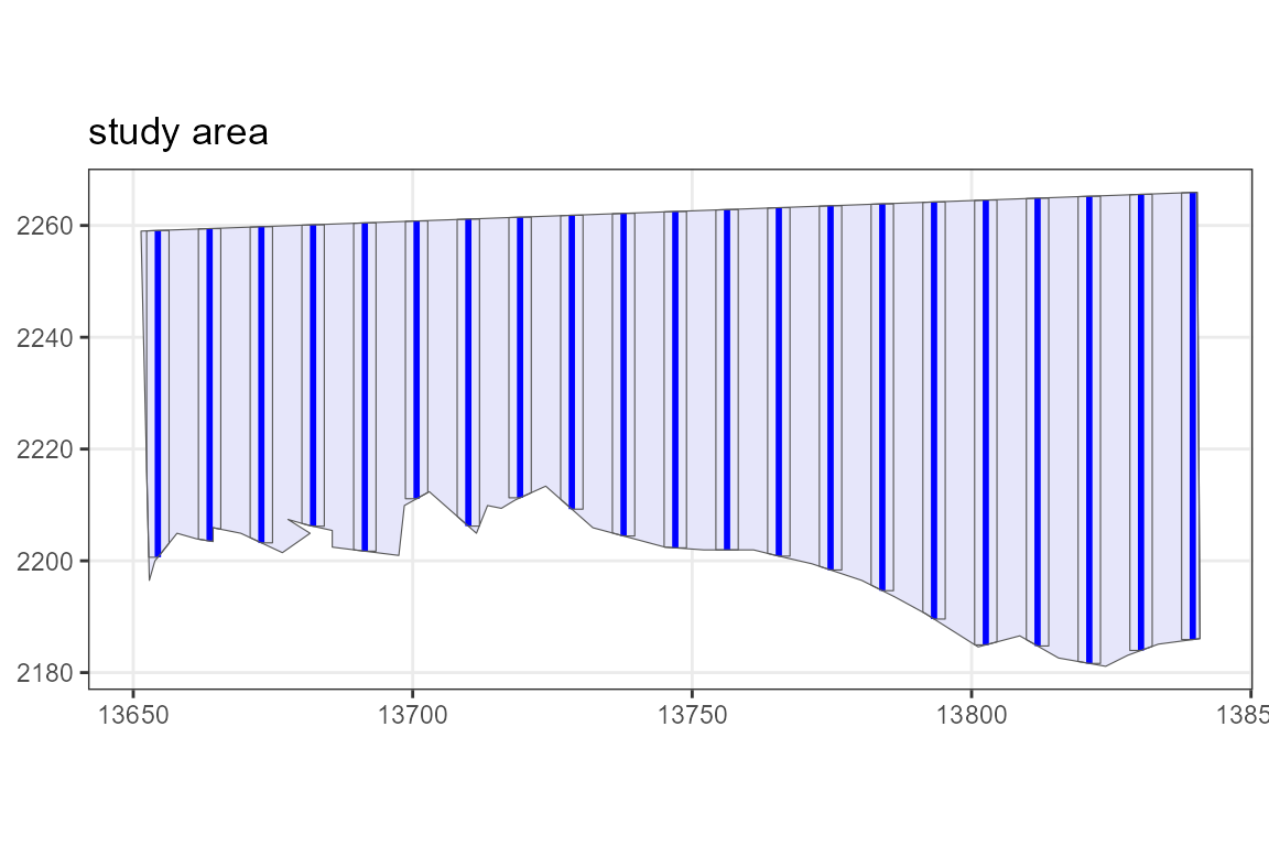
Figure 3: An example set of transects generated from the design along with the covered area shown by the black rectangles around the transects.
Assessing Coverage Uniformity and Design Statistics
Once we have checked that our design appears to be correctly specified we can assess how uniform the coverage is and also how values such as total line length, trackline length and cyclic trackline length vary across many surveys generated from our design. While we were given single values for these statistics from our one survey above it is important to check that all potential surveys from our design can be completed in the effort available, i.e. the maximum trackline/cyclic trackline length from the simulation should be achievable within the limits of the study. It is not permissible to generate more than one set of transects for the final survey and select the set with shorter/longer trackline length as then the selection of transect locations will no longer be purely random.
Parallel line designs should give uniform coverage across the majority of the survey region. The only exception to this is around the edge of the study region when we are using minus sampling, as we are using here. We will assess the effects of this now via a simulation which will generate 999 sets of transects from our design.
design <- run.coverage(design, reps = 999)We can now view the coverage scores by plotting our design object.
plot(design, subtitle = "Systematic Parallel, line.length = 1300km")## old-style crs object detected; please recreate object with a recent sf::st_crs()
## old-style crs object detected; please recreate object with a recent sf::st_crs()
## old-style crs object detected; please recreate object with a recent sf::st_crs()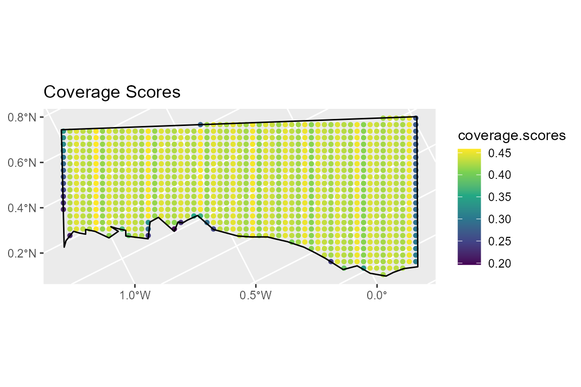
Figure 4: The coverage grid
The plot above indicates that coverage is fairly uniform over the majority of the study region. There are a few points around the edge of the survey region which have lower coverage than the others due to the minus sampling protocol, however for this example we would expect the effects of non-uniform coverage on the study estimates to be very small. The coverage grid points with lower coverage are very few in number and represent a very small proportion of the study region area.
We can also look at the design statistics, these are shown below.
design##
## Strata study area:
## ___________________
## Design: systematically spaced transects
## Spacing: NA
## Number of samplers: NA
## Line length: 1300 (shared across strata)
## Design angle: 0
## Edge protocol: minus
##
## Strata areas: 12037
## Region and effort units: km
## Coverage Simulation repetitions: 999
##
## Number of samplers:
##
## study area Total
## Minimum 20.0 20.0
## Mean 20.5 20.5
## Median 20.0 20.0
## Maximum 21.0 21.0
## sd 0.5 0.5
##
## Covered area:
##
## study area Total
## Minimum 5050.77 5050.77
## Mean 5147.14 5147.14
## Median 5101.63 5101.63
## Maximum 5310.94 5310.94
## sd 90.43 90.43
##
## % of region covered:
##
## study area Total
## Minimum 41.96 41.96
## Mean 42.76 42.76
## Median 42.38 42.38
## Maximum 44.12 44.12
## sd 0.75 0.75
##
## Line length:
##
## study area Total
## Minimum 1268.02 1268.02
## Mean 1299.52 1299.52
## Median 1282.34 1282.34
## Maximum 1348.13 1348.13
## sd 31.17 31.17
##
## Trackline length:
##
## study area Total
## Minimum 1450.50 1450.50
## Mean 1485.09 1485.09
## Median 1463.06 1463.06
## Maximum 1538.98 1538.98
## sd 35.32 35.32
##
## Cyclic trackline length:
##
## study area Total
## Minimum 1637.21 1637.21
## Mean 1672.06 1672.06
## Median 1649.37 1649.37
## Maximum 1724.80 1724.80
## sd 35.20 35.20
##
## Coverage Score Summary:
## ## old-style crs object detected; please recreate object with a recent sf::st_crs()
## old-style crs object detected; please recreate object with a recent sf::st_crs()
## old-style crs object detected; please recreate object with a recent sf::st_crs()
## old-style crs object detected; please recreate object with a recent sf::st_crs()
## old-style crs object detected; please recreate object with a recent sf::st_crs()
## old-style crs object detected; please recreate object with a recent sf::st_crs()
## old-style crs object detected; please recreate object with a recent sf::st_crs()
## old-style crs object detected; please recreate object with a recent sf::st_crs()## study area Total
## Minimum 0.19619620 0.19619620
## Mean 0.42611584 0.42611584
## Median 0.43243243 0.43243243
## Maximum 0.45845846 0.45845846
## sd 0.03585962 0.03585962First you are given a summary of the design, systematically spaced transects where the spacing was to be selected to achieve around 1300 km of effort. The lines were to be placed on a design angle of 0 and a minus sampling protocol was to be used.
We are then told the area of the study region, the units of the region coordinates and how many times the coverage simulation was repeated.
We now move on to the summary statistics from the 999 sets of transects generated during the simulation. We are told that each survey has between 20 and 21 samplers and that the minimum and maximum covered areas are 5051 and 5311 km^2 which equate to 42.0% and 44.1% of the study area, respectively. The minimum on-effort line length is 1268 km and the maximum on-effort line length is 1348 km, with a mean value of very close to the 1300km requested. We are then given the minimum, mean, median, maximum and standard deviation values for the trackline and cyclic trackline lengths. The maximum values for these statistics should be used to ensure that any set of transects randomly generated from the design is achievable in the total effort available given any time and financial constraints of the survey.
Finally, we are given a summary of the coverage score values. If we have even coverage then we should see little variation in the coverage scores. The minimum coverage score is 0.20 and the maximum is 0.46 indicating that some small areas around the edge of the study region (as shown in Figure 4) are half as likely to be sampled as those within the main part of the study region. We are given an indication of the variability of the coverage scores in the standard deviation provided but it may also be useful to plot a histogram of the coverage scores, Figure 5. Again this looks fairly reassuring that the parts of the study with lower coverage do not represent a significant proportion of the study area. However, if we wanted to be really thorough we could run a simulation study using DSsim and test a worse case scenario, where density in these areas of lower coverage varied from the rest of the study region. If we were worried that this non-uniform coverage could cause significant bias we could switch to a plus sampling strategy.
hist(get.coverage(design), xlab = "Coverage Scores", main = "Histogram of Coverage Scores")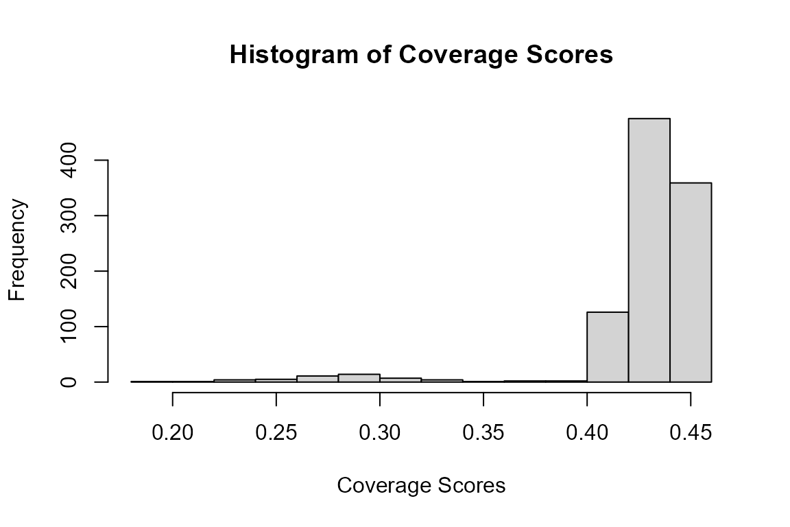
Figure 5: Histogram of coverage scores
Exporting transects
When you are confident that your design meets your survey objectives, you are ready to generate a final set of transects to use during your survey. To ensure that uniform coverage probability is maintained you must use the first randomly generated transect set. Regenerating transects due to an inconvenient transect property (e.g. intersection of an island or other feature / too few or too many samplers) will result in non-uniform coverage so must be avoided.
Once you have your final set of survey transects these can be exported in a number of formats. Below we demonstrate exporting the coordinates to shapefile and to csv file. See the write.transects help file for additional examples of exporting to .txt and .gpx. In the example below these files are written to a temporary directory, you will want to replace this with your own file path and name.
# File destination - .txt file
file.path <- paste0(tempdir(), "/", "transects.txt")
# Write to .txt file
write.transects(transects, dsn = file.path)


# File destination - .shp file
file.path <- paste0(tempdir(), "/", "transects.shp")
# Write to shapefile
write.transects(transects, dsn = file.path)
## writing: substituting ENGCRS["Undefined Cartesian SRS with unknown unit"] for missing CRS## Writing layer `transects' to data source
## `C:\Users\erexs\AppData\Local\Temp\RtmpcNG035/transects.shp' using driver `ESRI Shapefile'
## Writing 21 features with 2 fields and geometry type Line String.You can now navigate to your saved files and view their contents.
Appendix: Trackline and Cyclic Trackline Lengths
The following four figures (6 - 10) demonstrate how the trackline lengths and cyclic trackline lengths are calculated. The red arrows indicate the trackline path, moving from the start of the first transect along its length then across off effort to the next transect and so on until the end of the last transect is reached. The cyclic trackline length is then the trackline length represented by the red arrows plus the off effort transit time required to travel from the end of the last transect back to the beginning of the first as indicated by the light blue arrow. These values are provided to help you assess the efficiency of the design by comparing on-effort line length to total trackline length and also to help you ensure that the entire survey can be completed within time and budget constraints. Note that the trackline and cyclic trackline lengths for segmented designs are calculated in a very similar way to parallel line transect designs. The observer will start at the beginning of one segment and move up the line of segments before crossing to the next line of segments and so on.
