Plot fit of detection functions and histograms of data from distance sampling independent observer (io) model

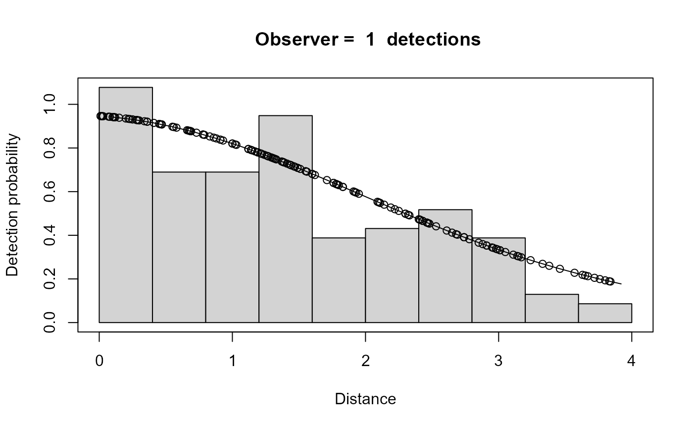
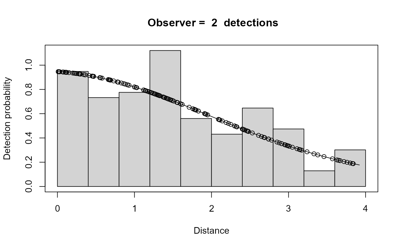
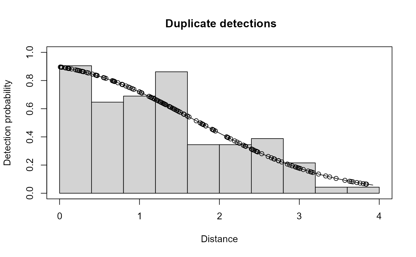
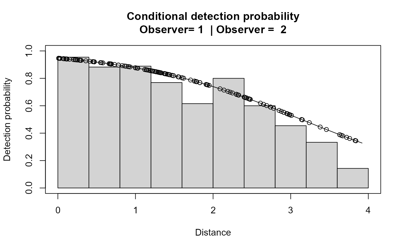
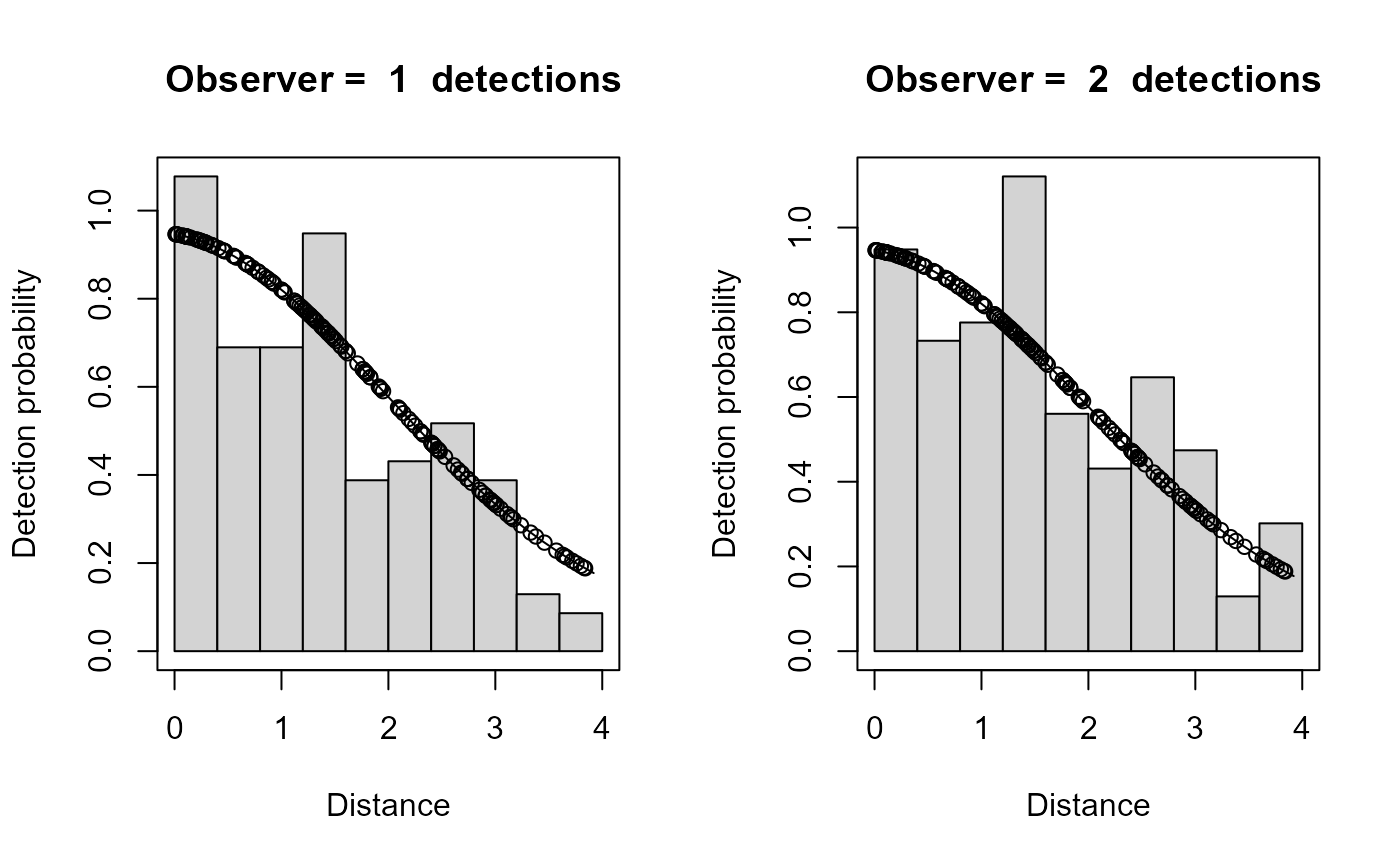
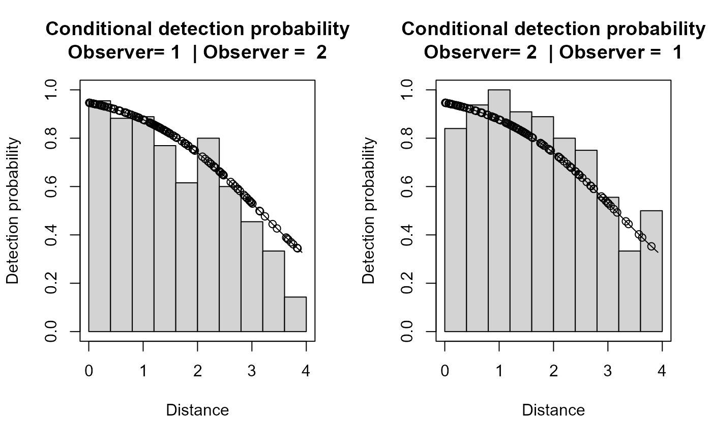
Plots the fitted detection functions for a distance sampling model and histograms of the distances (for unconditional detection functions) or proportion of observations detected within distance intervals (for conditional detection functions) to compare visually the fitted model and data.

Usage

# S3 method for class 'io'
plot(
  x,
  which = 1:6,
  breaks = NULL,
  nc = NULL,
  maintitle = "",
  showlines = TRUE,
  showpoints = TRUE,
  ylim = c(0, 1),
  angle = NULL,
  density = NULL,
  col = "lightgrey",
  jitter = NULL,
  divisions = 25,
  pages = 0,
  xlab = "Distance",
  ylab = "Detection probability",
  subtitle = TRUE,
  ...
)

Arguments

x

fitted model from ddf

which

index to specify which plots should be produced.

1	Plot primary unconditional detection function
2	Plot secondary unconditional detection function
3	Plot pooled unconditional detection function
4	Plot duplicate unconditional detection function
5	Plot primary conditional detection function
6	Plot secondary conditional detection function

Note that the order of which is ignored and plots are produced in the above order.

breaks

user define breakpoints

nc

number of equal-width bins for histogram

maintitle

main title line for each plot

showlines

logical variable; if TRUE a line representing the average detection probability is plotted

showpoints

logical variable; if TRUE plots predicted value for each observation

ylim

range of vertical axis; defaults to (0,1)

angle

shading angle for histogram bars.

density

shading density for histogram bars.

col

colour for histogram bars.

jitter

scaling option for plotting points. Jitter is applied to points by multiplying the fitted value by a random draw from a normal distribution with mean 1 and sd jitter.

divisions

number of divisions for averaging line values; default = 25

pages

the number of pages over which to spread the plots. For example, if pages=1 then all plots will be displayed on one page. Default is 0, which prompts the user for the next plot to be displayed.

xlab

label for x-axis

ylab

label for y-axis

subtitle

if TRUE, shows plot type as sub-title

...

other graphical parameters, passed to the plotting functions (plot, hist, lines, points, etc)

Value

Just plots

Details

The structure of the histogram can be controlled by the user-defined arguments nc or breaks. The observation specific detection probabilities along with the line representing the fitted average detection probability.

It is not intended for the user to call plot.io.fi but its arguments are documented here. Instead the generic plot command should be used and it will call the appropriate function based on the class of the ddf object.

Author

Jeff Laake, Jon Bishop, David Borchers, David L Miller

Examples

# \donttest{
library(mrds)
data(book.tee.data)
egdata <- book.tee.data$book.tee.dataframe
result.io <- ddf(dsmodel=~cds(key = "hn"), mrmodel=~glm(~distance),
                 data=egdata, method="io", meta.data=list(width=4))

# just plot everything
plot(result.io)







# Plot primary and secondary unconditional detection functions on one page
# and  primary and secondary conditional detection functions on another
plot(result.io,which=c(1,2,5,6),pages=2)


# }