Line transect density estimation

Eric Rexstad

CREEM, Univ of St Andrews

November 2024

In this exercise, we use R (R Core Team, 2019) and the Distance package (Miller, Rexstad, Thomas, Marshall, & Laake, 2019) to fit different detection function models to line transect survey data of winter wren (Troglodytes troglodytes) density and abundance. These data were part of a study described by Buckland (2006).

Objectives

• Fit a basic detection function using the ds function
• Plot and examine a detection function
• Fit different detection function forms.

Survey design

Nineteen line transects were walked twice (Figure 1).

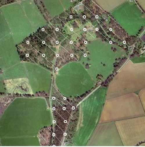
Figure 1: Montrave study area; diagonal lines indicate line transects walked to generate these data.

The fields of the wren_lt data set are:

• Region.Label - identifier of regions: in this case there is only one region and set to ‘Montrave’ required field
• Area - size of the study region (hectares): 33.2ha
• Sample.Label - line transect identifier (numbered 1-19) required field
• Effort - length of the line transects (km) required field
• object - unique identifier for each detected winter wren
• distance - perpendicular distance (metres) to each detection required field
• Study.Area - this is the name of the study, ‘Montrave 4’

Make the data available for R session

This command assumes that the Distance package has been installed on your computer. The R workspace wren_lt contains detections of winter wrens from the line transect surveys of Buckland (2006).

library(Distance)
data(wren_lt)

The effort, or transect length has been adjusted to recognise each transect is walked twice. Examine the first few rows of wren_lt using the function head()

head(wren_lt)

##   Region.Label Area Sample.Label Effort object distance Study.Area
## 1     Montrave 33.2            1  0.416      5       15 Montrave 4
## 2     Montrave 33.2            1  0.416      6       80 Montrave 4
## 3     Montrave 33.2            1  0.416      7       35 Montrave 4
## 4     Montrave 33.2            1  0.416      8       55 Montrave 4
## 5     Montrave 33.2            1  0.416     12       12 Montrave 4
## 6     Montrave 33.2            1  0.416     13       75 Montrave 4

The object wren_lt is a dataframe object made up of rows and columns.

sum(!is.na(wren_lt$distance))

## [1] 156

The code above determines the number of detection distances that are not missing. Why might there be rows in our data where detection distance is missing? Distance would have to be recorded as missing for rows representing transects on which there were no detections. The transect and its effort would need to appear in the data, but without detections, the perpendicular distance would be recorded as missing (NA).

Examine the distribution of detection distances

Gain familiarity with the perpendicular distance data using the hist() function (Figure 2).

hist(wren_lt$distance, xlab="Distance (m)", main="Winter wren line transects")

Figure 2: Distribution of perpendicular distances for winter wren from (Buckland, 2006).

Note that there appears to be too few detections between 0 and 20m, and too many detections between 20m and 40m. This may be evidence of evasive movement by winter wrens; see further discussion of this below.

Specify unit conversions

A guaranteed way to produce incorrect results from your analysis is to misspecify the units distances are measured. The ds function has an argument convert.units where the user provides a value to report density in proper units. Providing an incorrect value will result in estimates that are out by orders of magnitude.

We can choose the units in which winter wren density is to be reported, we choose square kilometre. How to transmit this information to the ds function?

The answer is another function convert_units. Arguments to this function are

• distance_units
  • units of measure for perpendicular/radial distances
• effort_units
  • units of measure for effort (NULL for point transects)
• area_units
  • units of measure for the study area.

Specify the correct arguments to this function for the winter wren data set. Note: units are specified as quoted strings, singular rather than plural; e.g. “meter” rather than “meters”

conversion.factor <- convert_units("meter", "kilometer", "hectare")

Fitting a simple detection function model with ds

Detection functions are fitted using the ds function and this function requires a data frame to have a column called distance. We have this in our nests data, therefore, we can simply supply the name of the data frame to the function along with additional arguments.

Details about the arguments for this function:

• key="hn"
  • fit a half-normal key detection function
• adjustment=NULL
  • do not include adjustment terms
• convert_units=conversion.factor
  • required because, for this example, the perpendicular distances are in metres and the line transect lengths are in kilometer - this argument converts the perpendicular distance measurements from metres to kilometer. Our density estimates will be reported in number of birds per hectare.

wren.hn <- ds(data=wren_lt, key="hn", adjustment=NULL, convert_units=conversion.factor)

On calling the ds function, information is provided to the screen reminding the user what model has been fitted and the associated AIC value. More information is supplied by applying the summary() function to the object created by ds().

summary(wren.hn)

## 
## Summary for distance analysis 
## Number of observations :  156 
## Distance range         :  0  -  100 
## 
## Model       : Half-normal key function 
## AIC         :  1418.188 
## Optimisation:  mrds (nlminb) 
## 
## Detection function parameters
## Scale coefficient(s):  
##             estimate        se
## (Intercept) 4.105816 0.1327744
## 
##                       Estimate          SE         CV
## Average p             0.685037  0.05678821 0.08289802
## N in covered region 227.724931 21.47275208 0.09429250
## 
## Summary statistics:
##     Region Area CoveredArea Effort   n  k       ER    se.ER      cv.ER
## 1 Montrave 33.2       193.2   9.66 156 19 16.14907 1.226096 0.07592366
## 
## Abundance:
##   Label Estimate       se        cv     lcl     ucl       df
## 1 Total 39.13286 4.399007 0.1124121 31.3023 48.9223 74.24595
## 
## Density:
##   Label Estimate        se        cv       lcl      ucl       df
## 1 Total   1.1787 0.1325002 0.1124121 0.9428403 1.473563 74.24595

The summary function

Examining the output produced by summary(wren.hn) notice

• number of detections used in fitting
• truncation distances
• AIC score
• parameters of the detection function (on a natural log scale)
• estimated probability of detection within the truncation distance
• estimated number of objects in the area covered by survey effort
• summary of the survey (effort, number of transects, number of detections)
  • encounter rate and its variability
• estimated abundance and density within the study area
  • and measures of precision
• if there are strata, estimates are provided for each stratum
• if objects were detected in groups, there are estimates of abundance of groups and of individuals

Visually inspect the fitted detection function with the plot() function, specifying the cutpoints histogram with argument breaks (Figure 3):

cutpoints <- c(0,5,10,15,20,30,40,50,65,80,100)
plot(wren.hn, breaks=cutpoints, main="Half normal model, wren line transects")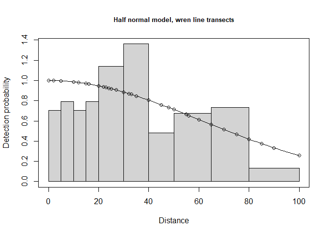

Figure 3: Fit of half normal detection function to wren data. Note large number of break points specified at small distances.

Continue to note the presence of evasive movement in this plot of the fit of detection function to the observed data.

Specifying different detection functions

Detection function forms and shapes, are specified by changing the key and adjustment arguments.

The options available for key detection functions are:

• half normal (key="hn") - default
• hazard rate (key="hr")
• uniform (key="unif")

The options available for adjustment terms are:

• no adjustment terms (adjustment=NULL)
• cosine (adjustment="cos") - default
• Hermite polynomial (adjustment="herm")
• Simple polynomial (adjustment="poly")

To fit a uniform key function with cosine adjustment terms, use the command:

wren.unif.cos <- ds(wren_lt, key="unif", adjustment="cos", convert_units=conversion.factor)

When this line of code is executed, multiple models will be fitted, successively adding addition adjustment terms. When the model with four adjustment terms is fit, an error message is returned; but a uniform key with 3 cosine adjustments is fitted and contained in the returned object.

AIC model selection will be used to fit adjustment terms of up to order 5.

To fit a hazard rate key function with simple polynomial adjustment terms, then use the command:

wren.hr.poly <- ds(wren_lt, key="hr", adjustment="poly", convert_units=conversion.factor)

Model comparison

Each fitted detection function produces a different estimate of winter wren abundance and density. The estimate depends upon the model chosen. The model selection tool for distance sampling data is AIC.

AIC(wren.hn, wren.hr.poly, wren.unif.cos)

##               df      AIC
## wren.hn        1 1418.188
## wren.hr.poly   2 1412.133
## wren.unif.cos  3 1416.430

df in the AIC table indicates the number of parameters associated with each model.

Absolute goodness of fit

In addition to the relative ranking of models provided by AIC, it is also important to know whether selected model(s) actually fit the data. The model is the basis of inference, so it is dangerous to make inference from a model that does not fit the data. Goodness of fit is assessed using the function gof_ds. This function by default, reports the goodness of fit assessed by the Cramer von-Mises test along with a quantile-quantile plot showing locations of deviations from good fit. Optionally, a \(\chi^2\) goodness of fit test and a bootstrap version of the Kolomogorov-Smirnov goodness of fit test can be performed. Using function defaults, we see results only of the Cramer von-Mises test along with the Q-Q plot (Figure 4).

gof_ds(wren.hr.poly)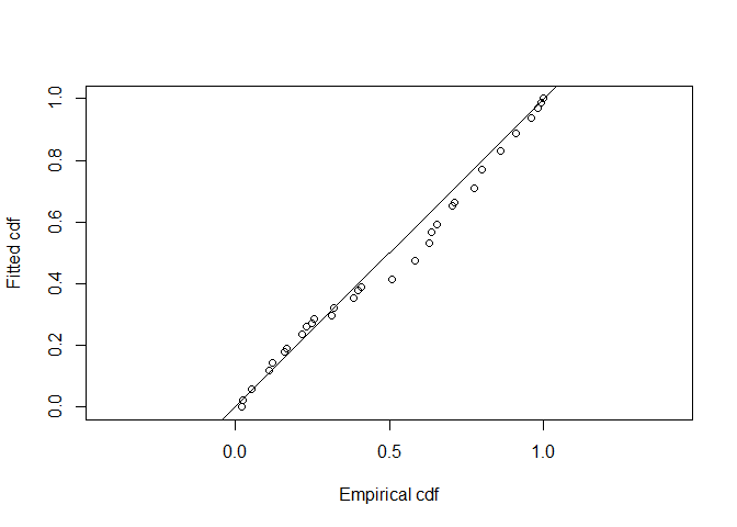

Figure 4: Q-Q plot of hazard rate key function fitted ot wren line transect data.

## 
## Goodness of fit results for ddf object
## 
## Distance sampling Cramer-von Mises test (unweighted)
## Test statistic = 0.249897 p-value = 0.188501

Even though there may have been evasive movement, the goodness of fit statistics are still sufficient for using detection function models for inference.

Model comparison tables

The function summarise_ds_models combines the work of AIC and gof_ds to produce a table of fitted models and summary statistics.

knitr::kable(summarize_ds_models(wren.hn, wren.hr.poly, wren.unif.cos),digits=3,
             caption="Model comparison table for wren line transect data, Montrave.")

Table 1: Model comparison table for wren line transect data, Montrave.

	Model	Key function	Formula	C-vM p-value	\(\hat{P_a}\)	se(\(\hat{P_a}\))	\(\Delta\)AIC
2		Hazard-rate	~1	0.189	0.844	0.025	0.000
3		Uniform with cosine adjustment terms of order 1,2,3	NA	0.198	0.757	0.140	4.298
1		Half-normal	~1	0.077	0.685	0.057	6.055

Model selection is not a cookbook

The AIC model selection tools suggest the hazard rate key function is the preferred model. However, examine the shape of the hazard rate detection function in contrast to the uniform cosine fitted detection function (Figure 5).

plot(wren.hr.poly, breaks=cutpoints, main="Hazard rate")
plot(wren.unif.cos, breaks=cutpoints, main="Uniform cosine")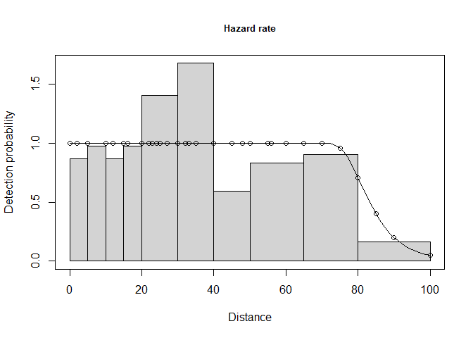

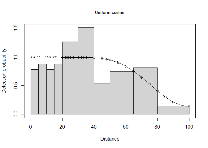
Figure 5: Possible evidence of evasive movement of wrens. Note left figure (hazard rate) with implausible perfect detectability out to 70m, then precipitous decline.

The fellow who gathered these data (Prof Buckland) maintained the shape of the fitted hazard rate detection function is not plausible. Instead, he chose the uniform key with cosine adjustments for making inference (Buckland, 2006, p. 352):

Common Chaffinch and Winter Wren showed some evidence of observer avoidance. For 2 of the 12 data sets, this resulted in a fitted hazard rate detection function with certain detection out to ∼60 m, with an implausibly rapid fall-off beyond 70 m. In these two analyses, a model with a slightly higher AIC value and a more plausible fit to the detection function was selected.

This is an example of moderating objective model selection tools with common sense and understanding of field procedures.

References

Buckland, S. T. (2006). Point transect surveys for songbirds: Robust methodologies. The Auk, 123(2), 345–345. https://doi.org/10.1642/0004-8038(2006)123[345:psfsrm]2.0.co;2

Miller, D. L., Rexstad, E., Thomas, L., Marshall, L., & Laake, J. L. (2019). Distance sampling in r. Journal of Statistical Software, 89(1), 1–28. https://doi.org/10.18637/jss.v089.i01

R Core Team. (2019). R: A language and environment for statistical computing. Vienna Austria: R Foundation for Statistical Computing.