Variance estimation

Continuing with the Montrave winter wren line transect data from the line transect vignette, we focus upon producing robust estimates of precision in our point estimates of abundance and density. The analysis in R (R Core Team, 2019) makes use of the Distance package (Miller, Rexstad, Thomas, Marshall, & Laake, 2019).

Objectives

Estimate precision in the standard manner
Use the bootstrap to estimate precision
Incorporate model uncertainty in our estimates of precision

Survey data

The R workspace wren_lt contains detections of winter wrens from the line transect surveys of S. T. Buckland (2006).

library(Distance)
data(wren_lt)

The function names() allows you to see the names of the columns of the data frame wren_lt. Definitions of those fields were provided in the line transect vignette.

The effort, or transect length has been adjusted to recognise each transect is walked twice.

conversion.factor <- convert_units("meter", "kilometer", "hectare")

Fitting a suitable detection function

Rather than refitting models used in the line transect vignette, we move directly to the model selected by S. T. Buckland (2006).

wren.unif.cos <- ds(wren_lt, key="unif", adjustment="cos",
                  convert_units=conversion.factor)

Based upon experience in the field, the uniform cosine model was used for inference.

Estimation of precision

Looking at the density estimates from the uniform cosine model

print(wren.unif.cos$dht$individuals$D)

##   Label Estimate        se        cv       lcl      ucl      df
## 1 Total 1.066101 0.2126892 0.1995019 0.7218009 1.574632 168.204

The coefficient of variation (CV) is 0.2, and confidence interval bounds are (0.72 - 1.57) birds per hectare. The coefficient of variation is based upon a delta-method approximation of the uncertainty in both the parameters of the detection function and the variability in encounter rates between transects.

\[[CV(\hat{D})]^2 = [CV(\frac{n}{L})]^2 + [CV(P_a)]^2\] where

$n$ is number of detections
$L$ is total effort
$P_a$ is probability of detection given a bird is within the covered region.

These confidence interval bounds assume the sampling distribution of $\hat{D}$ is log-normal (S. Buckland, Rexstad, Marques, & Oedekoven, 2015, sec. 6.2.1).

Bootstrap estimates of precision

Rather than relying upon the delta-method approximation that assumes independence between uncertainty in the detection function and variability in encounter rate, a bootstrap procedure can be employed. Resampling with replacement of the transects produces replicate samples with which a sampling distribution of $\hat{D}$ is approximated. From that sampling distribution, the percentile method is used to produce confidence interval bounds respecting the shape of the sampling distribution (S. Buckland et al., 2015, sec. 6.3.1.2).

The function bootdht_Nhat_summarize is included in the Distance package. It is used to extract information from the object created by bootdht. I will modify it slightly so as to extract the density estimates rather than the abundance estimates.

bootdht_Dhat_summarize <- function(ests, fit) {
  return(data.frame(D=ests$individuals$D$Estimate))
}

After the summary function is defined, the bootstrap procedure can be performed. Arguments here are the name of the fitted object, the object containing the data, conversion factor and number of bootstrap replicates. Here, I use the cores= argument to use multiple cores to process the bootstraps in parallel. If you do not have this many cores in your computer, you will need to reduce/remove the argument.

nboots <- 300
est.boot <- bootdht(model=wren.unif.cos, flatfile=wren_lt,
                    summary_fun=bootdht_Dhat_summarize,
                    convert_units=conversion.factor, nboot=nboots, cores=10)

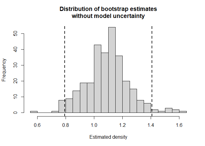
The object est.boot contains a data frame with two columns consisting of $\hat{D}$ as specified in bootdht_Dhat_summarize. This data frame can be processed to produce a histogram (Fig. 1) representing the sampling distribution of the estimated parameters as well as the percentile confidence interval bounds.

alpha <- 0.05
(bootci <- quantile(est.boot$D, probs = c(alpha/2, 1-alpha/2), na.rm=TRUE))

##      2.5%     97.5% 
## 0.7940937 1.4088653

hist(est.boot$D, nc=30,
     main="Distribution of bootstrap estimates\nwithout model uncertainty",
     xlab="Estimated density")
abline(v=bootci, lwd=2, lty=2)

$Sampling distribution of $\hat{D}$ approximated from bootstrap.$

Figure 1: Sampling distribution of $\hat{D}$ approximated from bootstrap.

Incorporating model uncertainty in precision estimates

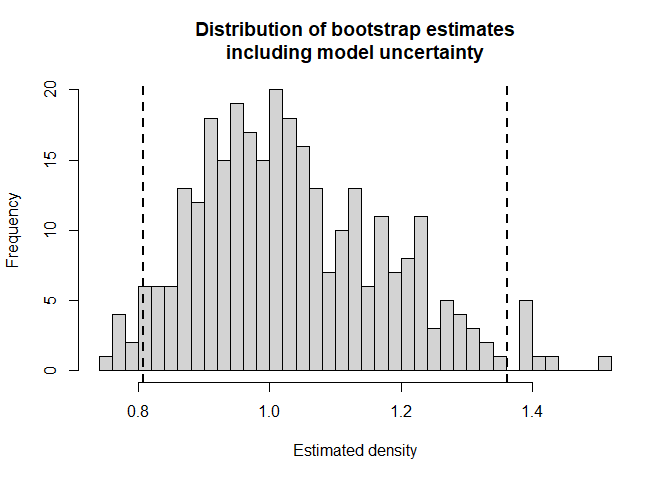
The argument model in bootdht can be a single model as shown above, or it can consist of a list of models. In the later instance, all models in the list are fitted to each bootstrap replicate and model selection based on AIC is performed for each replicate. The consequence is that model uncertainty is incorporated into the resulting estimate of precision (Fig. 2).

wren.hn <- ds(wren_lt, key="hn", adjustment="cos",
                  convert_units=conversion.factor)

## Warning in check.mono(result, n.pts = control$mono.points): Detection function
## is not strictly monotonic!
## Warning in check.mono(result, n.pts = control$mono.points): Detection function
## is not strictly monotonic!

wren.hr.poly <- ds(wren_lt, key="hr", adjustment="poly",
                  convert_units=conversion.factor)
est.boot.uncert <- bootdht(model=list(wren.hn, wren.hr.poly, wren.unif.cos), 
                           flatfile=wren_lt,
                           summary_fun=bootdht_Dhat_summarize,
                           convert_units=conversion.factor, nboot=nboots, cores=10)

(modselci <- quantile(est.boot.uncert$D, probs = c(alpha/2, 1-alpha/2), na.rm=TRUE))

##      2.5%     97.5% 
## 0.8080775 1.3620822

hist(est.boot.uncert$D, nc=30, 
     main="Distribution of bootstrap estimates\nincluding model uncertainty",
     xlab="Estimated density")
abline(v=modselci, lwd=2, lty=2)

$Sampling distribution of $\hat{D}$ approximated from bootstrap including model uncertainty.$

Figure 2: Sampling distribution of $\hat{D}$ approximated from bootstrap including model uncertainty.

Comments

Recognise that producing bootstrap estimates of precision is computer-intensive. In this example we have created only 300 bootstrap replicates in the interest of computation time. For inference you wish to draw, you will likely increase the number of bootstrap replicates to 999.

For this data set, the bootstrap estimate of precision is greater than the delta-method approximation precision (based on confidence interval width). In addition, incorporating model uncertainty into the estimate of precision for density changes the precision estimate very little. The confidence interval width without incorporating model uncertainty is 0.615 while the confidence interval including model uncertainty is 0.554. This represents a change of -10% due to uncertainty regarding the best model for these data.

References

Buckland, S. T. (2006). Point transect surveys for songbirds: Robust methodologies. The Auk, 123(2), 345–345. https://doi.org/10.1642/0004-8038(2006)123[345:psfsrm]2.0.co;2

Buckland, S., Rexstad, E., Marques, T., & Oedekoven, C. (2015). Distance sampling: Methods and applications. Springer.

Miller, D. L., Rexstad, E., Thomas, L., Marshall, L., & Laake, J. L. (2019). Distance sampling in r. Journal of Statistical Software, 89(1), 1–28. https://doi.org/10.18637/jss.v089.i01

R Core Team. (2019). R: A language and environment for statistical computing. Vienna Austria: R Foundation for Statistical Computing.

Eric Rexstad

November 2024