Solving the size bias problem

In this example we have a sample of sightings data from eastern tropical Pacific (ETP) offshore spotted dolphin, collected by observers board tuna vessels (the data were made available by the Inter-American Tropical Tuna Commission - IATTC). More details about surveys of dolphins in the ETP can be found in T. Gerrodette & Forcada (2005) and Tim Gerrodette (2008). In the ETP, schools of yellow fin tuna commonly associate with schools of certain species of dolphins, and so vessels fishing for tuna often search for dolphins in the hopes of also locating tuna. For each school detected by the tuna vessels, the observer records the species, sighting angle and distance (later converted to perpendicular distance and truncated at 5 nautical miles), school size, and a number of covariates associated with each detected school.

A variety of search methods were used to find the dolphins from these tuna vessels. The coding in the data set is shown below.

Table 1: Table 2: Search method coding from tuna vessels in ETP.
Method	code
Crows nest	0
Bridge	2
Helicopter	3
Radar	5

Some of these methods may have a wider range of search than the others, and so it is possible that the detection function varies according to the method being used.

For each sighting the initial cue type is recorded. This may be birds flying above the school, splashes on the water, floating objects such as logs, or some other unspecified cue.

Table 3: Table 4: Cue coding from tuna vessels in ETP.
Cue	code
Birds	1
Splashes	2
Unspecified cue	3
Floating objects	4

Another covariate that potentially affects the detection function is sea state. Beaufort levels are grouped into two categories, the first including Beaufort values ranging from 0 to 2 (coded as 1) and the second containing values from 3 to 5 (coded as 2).

The sample data encompasses sightings made over a three month summer period.

Table 5: Table 6: Month coding from tuna vessels in ETP.
Month	code
June	6
July	7
August	8

Prepare data for analysis

Exploratory data analysis

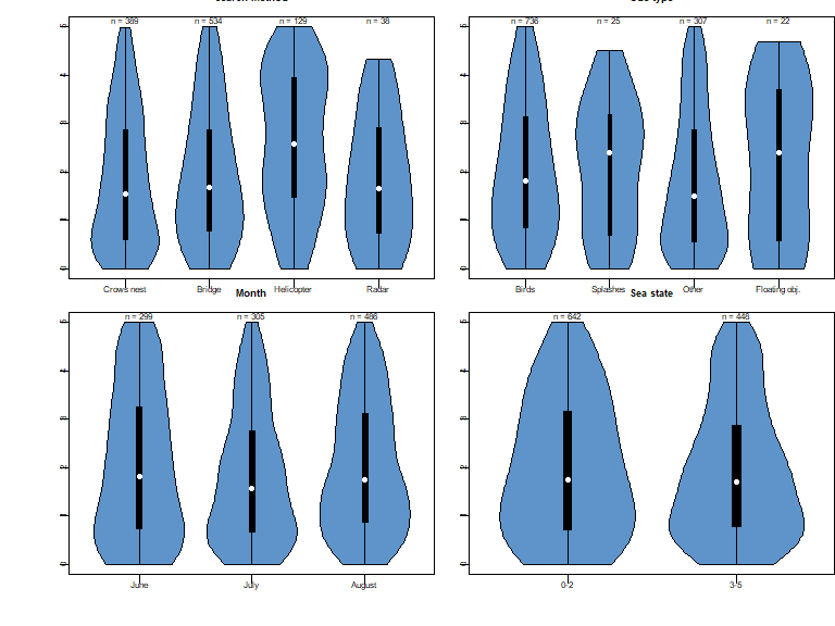
As described, there are a number of potential covariates that might influence dolphin detectability. Rather than throw all covariates into detection function models, examine the distribution of detection distances (y-axis of figure below) as a function of the plausible factor covariates.

Figure 1: Exploratory data analysis using violin plots. Prepared using the vioplot package. Number of detections show above plots.

From Fig. 1 there are several decisions to be made concerning the remaining analysis:

there is no discernible effect of month or sea state upon distribution of detection distances in this data set. Those covariates will not feature in subsequent modelling.
the distribution of detection distances by cue type appears to differ for splashes and floating objects. However, the number of detections associated with splash (n=25) or float objects (n=22) cues is small, accounting for ~4% of the total number of detections. I choose to ignore variability in detection probability associated with cue type.
shape of the distribution of detections likely does change for the different search methods. However, the method for which detection distances are most different is the helicopter. The violin plot shows there to be roughly an equal number of pods detected between 4 and 5 nautical miles as were detected between 0 and 1 nautical miles.
- the proper way to handle this situation would be to remove helicopter sightings from the detection function modelling. Detectability could be assumed perfect out to the truncation distance, hence treat the helicopter portion of the survey as a strip transect. The number of pods detected by helicopters could be added into the estimated number of pods within the covered area. We will remove detections by helicopter from the remainder of our analysis.
the number of detections by radar is small and unlikely to exert much influence upon detection function modelling.

Evidence for size bias

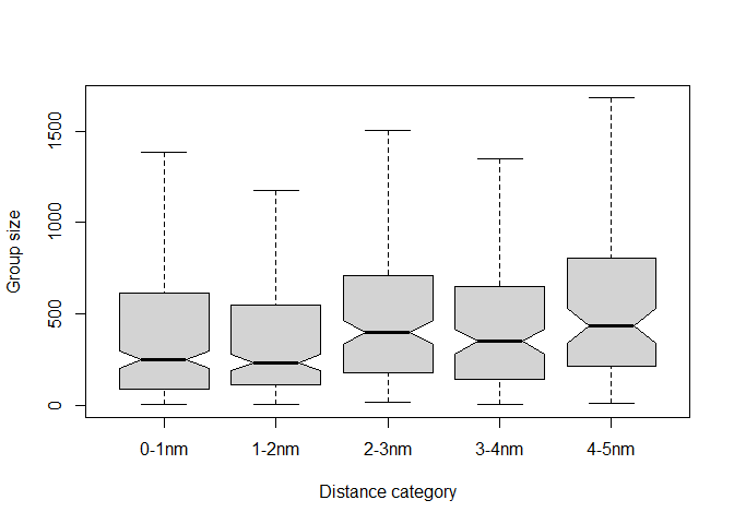
Size bias (Buckland et al., 2001) can be examined by plotting distribution of group size as a function of detection distances.

Box plot of observed group sizes by perpendicular distance band. Outliers are not shown; notches indicate discernable difference in mean group size at 2nm.

Figure 2: Box plot of observed group sizes by perpendicular distance band. Outliers are not shown; notches indicate discernable difference in mean group size at 2nm.

Fig. 2 indicates a difference in observed mean group size at 2nm; with average group size being distinctly larger at distances greater than 2nm. Hence, average group size in the sample is an overestimate of the average group size in the population. Our modelling of the detection function will need to counteract this bias by including group size in the detection function.

Stage one of detection function modelling

Before creating a host of candidate models, we should address with the question of the appropriate key function for these data. Recall we are not including sightings made from the helicopter platform in our analyses.

Fitting models with half normal key function without adjustments and with and without Search.method

hn <- ds(nochopper, key="hn", adjustment = NULL)
hn.method <- ds(nochopper, key="hn", formula = ~factor(Search.method))
par(mfrow=c(1,2))
gof_ds(hn, main="HN key, no adj", cex=0.5)

## 
## Goodness of fit results for ddf object
## 
## Distance sampling Cramer-von Mises test (unweighted)
## Test statistic = 0.656421 p-value = 0.0162635

gof_ds(hn.method, main="HN key + method", cex=0.5)

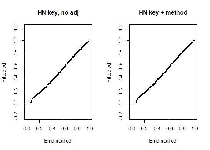
Figure 3: Q-Q goodness of fit plots for half normal key function without adjustments also including search method as a covariate.

## 
## Goodness of fit results for ddf object
## 
## Distance sampling Cramer-von Mises test (unweighted)
## Test statistic = 0.672219 p-value = 0.0148816

par(mfrow=c(1,2))

indicates a lack of fit of the half normal key function models. After some rounding to the trackline, the detection function maintains a shoulder before falling away quite rapidly. Even taking into consideration the idea that the sample size is very large (n=961), making the goodness of fit test quite powerful, there is some doubt that the half normal key function is appropriate for these data. We will remove the half normal from further modelling, as the hazard rate will serve our purposes, as the hazard rate without adjustments or covariates, adequately fit the data.

hr <- ds(nochopper, key="hr")

## Starting AIC adjustment term selection.

## Fitting hazard-rate key function

## AIC= 2920.797

## Fitting hazard-rate key function with cosine(2) adjustments

## Warning in check.mono(result, n.pts = control$mono.points): Detection function
## is greater than 1 at some distances
## Warning in check.mono(result, n.pts = control$mono.points): Detection function
## is greater than 1 at some distances

## AIC= 2922.8

## 
## Hazard-rate key function selected.

gof_ds(hr, plot=FALSE)

## 
## Goodness of fit results for ddf object
## 
## Distance sampling Cramer-von Mises test (unweighted)
## Test statistic = 0.130299 p-value = 0.455606

Counteracting size bias

Conducting our modeling using the hazard rate key function, we turn our attention to incorporating group size into the detection function. The way to counteract the effect of size bias is to include group size in the detection function.

hr.size <- ds(nochopper, key="hr", formula = ~size)

## Model contains covariate term(s): no adjustment terms will be included.

## Fitting hazard-rate key function

## AIC= 2919.357

It is a disappointment to learn that a model including group size as a covariate fails to converge. There are numerical difficulties associated with a covariate that spans three orders of magnitude. For more about fitting issues with covariates, consult the covariate example with amakihi.

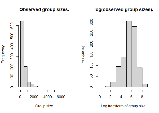
The distribution of group sizes is strongly skewed to the right, with a very long right tail. A transformation by natural logs will both reduce the range of log(size) to one order of magnitude and shift the centre of the distribution of the covariate (Fig. 4).

Figure 4: Effect of log transformation upon distribution of observed group sizes.

The convergence problems associated with using size as a covariate in the detection function are alleviated as a result of the transformation.

hr.clus <- ds(nochopper, key="hr", formula = ~log(size))

## Model contains covariate term(s): no adjustment terms will be included.

## Fitting hazard-rate key function

## AIC= 2904.307

Having successfully incorporated group size into the detection function, we proceed to examine the consequence of using Search.method as a covariate and a model incorporating both covariates.

hr.method <- ds(nochopper, key="hr", formula = ~factor(Search.method))
hr.clus.method <- ds(nochopper, key="hr", formula = ~log(size) + factor(Search.method))

Table 7: Table 8: Models with hazard rate key function fitted to tuna fishing vessel sightings of dolphins. Sightings from helicopter not included in modelling.
Key function	Formula	C-vM p-value	\(\hat{P_a}\)	se(\(\hat{P_a}\))	\(\Delta\)AIC
Hazard-rate	~log(size)	0.465	0.551	0.035	0.000
Hazard-rate	~log(size) + factor(Search.method)	0.458	0.547	0.036	2.604
Hazard-rate	~1	0.456	0.564	0.036	16.490
Hazard-rate	~factor(Search.method)	0.463	0.553	0.037	18.232

Interpretation of findings

All of the fitted models using the hazard rate as the key function fit the data. In addition, note the estimates of \(\widehat{P_a}\) for all four models. Inclusion of covariates has a negligible effect upon estimated detection probability. Despite a \(\Delta\)AIC value > 15, the model without covariates produces a virtually identical estimate of detection probability. This is another example of the remarkable property of pooling robustness of distance sampling estimators (Rexstad, Buckland, Marshall, & Borchers, 2023).

We discuss estimates of group and individual density from this data set. However, this data set does not accurately reflect survey effort. The Effort column is filled with 1 and there is only a single transect labelled in the data. Hence, the density estimates do not reflect biological reality; nevertheless the comparisons between models are legitimate. Variability between transects is also not properly incorporated into this analysis, so I won’t present measures of precision associated with any of the following point estimates.

This slight variation in \(\widehat{P_a}\) among the hazard rate candidate models is reflected in the equally similar estimates of dolphin pod density among the competing models. The model with the largest \(\widehat{P_a}\) produces the lowest estimate of \(\widehat{D_s}\) (170.5); while the model with the smallest \(\widehat{P_a}\) produces the largest estimate of \(\widehat{D_s}\) (175.8).

However, the most important consideration in analysis of this data set is proper treatment of size bias. The hazard rate models without group size in the detection function, estimate average group size in the population to be 515 whereas the model incorporating group size in the detection function estimates average group size in the population to be 408. Based on the evidence presented in Fig. 2, there is reason to believe that estimates of average group size without incorporating group size in the detection function results in a positively biased estimate of group size in the population. From the group size estimates under the two models, it appears the magnitude of that positive size bias in this data set is 26.2.

This difference in estimated average group size is magnified in the estimates of individual density \(\widehat{D_I}\). The model without covariates estimates \(\widehat{D_I}\) = 87805 while the model with group size as a covariate estimates \(\widehat{D_I}\) to be 71150.

Summary

Take home points:

Before incorporating covariates into the detection function, do a thorough exploratory data analysis with lots of plots.
Make at least a preliminary decision regarding key functions to consider before building an extensive candidate model set.
For this data set, there is little difference in the fit of the detection functions through the inclusion of covariates (pooling robustness).
However, exploratory data analysis suggested that small dolphin groups were missed at large distances, resulting in size bias in the estimate of average group size in the population.
Incorporating group size as a covariate in the detection function reduced the estimate group size in the population by 26.2%. This reduction in estimated group size compensated for the size bias induced by the detection process.

References

Buckland, S. T., Anderson, D. R., Burnham, K. P., Laake, J. L., Borchers, D. L., & Thomas, L. (2001). Introduction to distance sampling: Estimating abundance of biological populations. Oxford, New York: Oxford University Press.

Gerrodette, Tim. (2008). Estimates of 2006 dolphin abundance in the eastern tropical pacific, with revised estimates from 1986-2003. NOAA-TM-NMFS-SWFSC;422.

Gerrodette, T., & Forcada, J. (2005). Non-recovery of two spotted and spinner dolphin populations in the eastern tropical pacific ocean. Marine Ecology Progress Series, 291, 1–21. https://doi.org/10.3354/meps291001

Rexstad, E., Buckland, S., Marshall, L., & Borchers, D. (2023). Pooling robustness in distance sampling: Avoiding bias when there is unmodelled heterogeneity. Ecology and Evolution, 13(1), e9684. https://doi.org/10.1002/ece3.9684

Eric Rexstad

November 2024