Detecting density estimate differences
Eric Rexstad
CREEM, Univ of St AndrewsSeptember 2025
Source:vignettes/web-only/differences/differences.Rmd
differences.RmdManagement context
Often ecological questions extend beyond simply wanting an estimate of density in a study region. It is common for inference to extend to differences in density over time or space.
Conventional analysis
In Buckland et al. (2001, Sect. 3.6.5) methods are described to produce tests of significance based on t-test methods. That section presents formulas for comparing two density estimates under two scenarios
- the two estimates have separate detection functions, or
- the estimates share a common detection function.
The situation that Buckland et al. (2001) does not consider is the situation in which the two estimates are linked via a covariate in the detection function. Because the t-test framework cannot deal with this intermediate situation, an alternative approach, employing the bootstrap, can be employed. The bootstrap provides the added advantage that no parametric assumptions (t-distribution) need to be invoked when making inference.
Bootstrap analysis
A function in the Distance R package (Miller, Rexstad, Thomas, Marshall, & Laake, 2019) exists for computing uncertainty in density estimates via bootstrapping. This vignette demonstrates a function that harnesses the bootdht function to produce a sampling distribution of the difference between pairs of density estimates embedded as strata within a data set.
Recognise that strata can represent not only geographic divisions of a study area, but potentially also a survey of the same study area at another time. If a data set is organised in this manner, then the assessment of differences between strata would be an assessment of the possible change in density over time. Furthermore, as shown in the example of multi-species surveys, species could serve as strata. In this context, assessing the difference in stratum-specific density would examine the difference in density between species.
#' @title differences.bootstrap
#'
#' @description Test for pairwise density differences between strata
#'
#' Test is performed by producing replicate stratum-specific estimates and calculating
#' differences of each replicate.  Differencing is done for all pairs of strata in
#' the survey, e.g. if there are 4 strata there are \code{choose(4,2)=6} pairwise
#' comparisons computed.
#'
#' Histograms are produced for each comparison, designating the median of the distribution
#' and a percentile-based 95% confidence interval from the sampling distribution
#'
#' Difficulties can arise from very long left or right tails of the distribution
#' resulting from awkward bootstrap replicates.  The limits of the histogram are
#' cut off at 5*median so histogram shape does not appear degenerate. Code presumes differences will be positive.
#'
#' @param dsobj dsmodel object generated by \code{ds}
#' @param flatfile flatfile of survey data analysed by \code{ds}
#' @param nboot number of bootstrap replicates to compute
#'
#' @return Histogram showing sampling distribution of differences plus named list
#' \itemize{
#'   \item medians - median of sampling distribution
#'   \item ps - P-value for two-tailed test that difference is zero
#'   \item thematrix - Matrix of replicate pairwise differences
#' }
#' @importFrom Distance bootdht
#' @export
#'
#' @examples
#' library(Distance)
#' data(minke)
#' hn.pooled <- ds(minke)  # pooled detection function with hn key
#' result <- differences.bootstrap(hn.pooled, minke, nboot=100)
differences.bootstrap <- function(dsobj, flatfile, nboot) {

  num.strata <- length(dsobj$dht$individuals$D$Estimate) - 1
  stopifnot(
    'first argument is not a dsmodel object'           = class(dsobj) == 'dsmodel',
    'study area must have >1 stratum'                  = num.strata > 1,
    'specified flatfile object is not a data.frame   ' = class(flatfile) == 'data.frame'
  )
  d.point.ests <- dsobj$dht$individuals$D$Estimate
  strata.names <- dsobj$dht$individuals$D$Label
#   Following function used by bootdht to collect density point estimates
#     from each bootstrap replicate
  pullout.D <- function(ests, fit) {
    bill <- ests$individuals$D$Estimate
    extract <- data.frame(t(bill))
    colnames(extract) <- ests$individuals$D$Label
    return(extract)
  }
  outcome <- bootdht(dsobj, flatfile=flatfile, cores=10,
                     summary_fun=pullout.D, nboot=nboot)
#   Having run the bootstrap, calculate number of pairwise comparisons btwn strata
#     create objects to receive the replicate-wise differences for each comparison
#     median differences are reported and empirical P-value computed for each comparison
#     histograms of sampling distribution for differences are shown with CIs
#  allstrata <- complete.cases(outcome)
  num.compare <- choose(num.strata, 2)
  pairs <- t(combn(1:num.strata, 2))
  result.matrix <- matrix(data=NA, nrow=nrow(outcome), ncol=num.compare)
  themedian <- array(data=NA, dim=num.compare)
  pvalue <- array(data=NA, dim=num.compare)
  par(mfrow=c(num.compare, 1))
  for (i in 1:num.compare) {
    result.matrix[,i] <- mapply('-', outcome[pairs[i,2]], outcome[pairs[i,1]])
    themedian[i] <- median(result.matrix[,i], na.rm=TRUE)
    pvalue[i] <- ifelse(themedian[i]>0,
                        sum(result.matrix[,i]<0, na.rm=TRUE) / sum(!is.na(result.matrix[ ,i])),
                        sum(result.matrix[,i]>0, na.rm=TRUE) / sum(!is.na(result.matrix[ ,i])))
    tmp <- result.matrix[ ,i]
    hist(tmp[abs(tmp)<5*abs(themedian[i])],
         breaks=30, xlab="Estimated difference",
         main=paste("Bootstrap test of equality of two density estimates",
                    "\nMedian difference=", round(themedian[i],4),
                    " Two-tailed P-value=", round(2*pvalue[i],4)))
    abline(v=themedian[i])
    abline(v=quantile(result.matrix[,i], probs = c(0.025, 0.975), na.rm=TRUE), lty=3)
    first <- pairs[i, 1]
    second <- pairs[i, 2]
    line1 <- bquote(hat(D)[.(strata.names[first])] == .(round(d.point.ests[first], 4)))
    line2 <- bquote(hat(D)[.(strata.names[second])] == .(round(d.point.ests[second], 4)))
    legend("topleft", legend=as.expression(c(line1, line2)))
  }
  par(mfrow=c(1,1))
  return(list(medians=themedian, ps=2*pvalue, thematrix=result.matrix))
}
Examples
Several examples of the use of differences.bootstrap are provided. They make use of data sets that are included in the Distance package.
Two strata with pooled detection function
The simplest example uses the minke data set that consists of two geographic strata (North and South). A model that can be fitted to these data assumes the two strata share a common detection function
library(Distance)
data(minke)
hr.pooled <- ds(minke, key="hr", truncation=1.5)
result <- differences.bootstrap(hr.pooled, flatfile=minke, nboot=250)
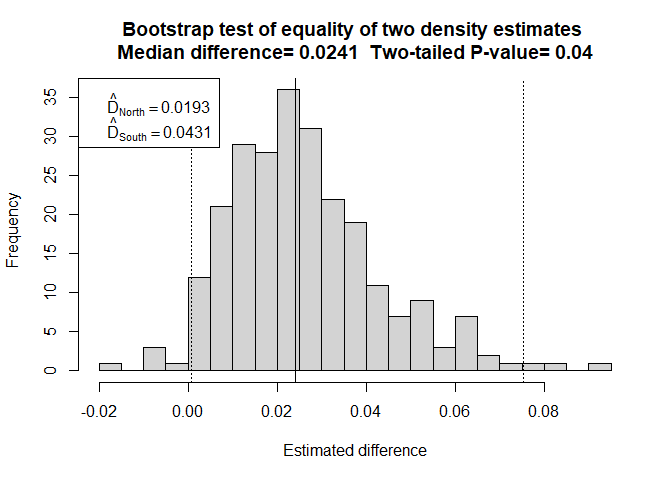
Figure 1: Strata share a pooled detection function.
Output from the function consists primarily of a histogram of the replicate density differences. This approximates the sampling distribution of the estimated density difference. A solid vertical line depicts the median of that distribution (medians are less influenced by outliers than are means). Dotted vertical lines depict the 95th percentiles around the estimated difference. The two-tailed P-value is presented in the histogram main title. In the legend box are presented the density estimates from the two strata, labelled using the Region.Label values found in the dsmodel object passed to the function.
Two strata with stratum as covariate
Working with the same minke data set, we present an alternative analysis in which stratum-specific detection functions are derived using stratum as a covariate in the detection function. Having fitted that detection function model to the data, the comparison of the densities in the strata are performed using the same function.
hr.covar <- ds(minke, key="hr", truncation=1.5, formula=~Region.Label)
resultcovar <- differences.bootstrap(hr.covar, flatfile=minke, nboot=250)
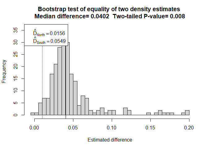
Figure 2: Two strata with Region.Label as a covariate in detection function.
The evidence that densities differ in the two strata appear stronger in this analysis because the dependence in the two estimates is reduced as a result of stratum-specific detection functions being used. Of course, inference would not be drawn from two different analyses of the same data set, this is merely to demonstrate the use of the function. If we were to perform model selection upon the two detection function models fitted to the minke data, we would find the model with stratum as a covariate is preferable and our inference should be based upon this second analysis.
Three strata with stratum as covariate
Another data set, Savannah_sparrow_1980, is derived from a point transect survey of a study area with three strata. We will fit a model with stratum as a covariate and send the result to our function to assess whether there are differences between the three strata.
data("Savannah_sparrow_1980")
hn.sparrow <- ds(Savannah_sparrow_1980, transect="point", key="hn", truncation="10%",
                 convert_units=convert_units("meter", NULL, "hectare"), formula=~Region.Label)
resultsparrow <- differences.bootstrap(hn.sparrow,
                                       flatfile=Savannah_sparrow_1980,
                                       nboot=250)
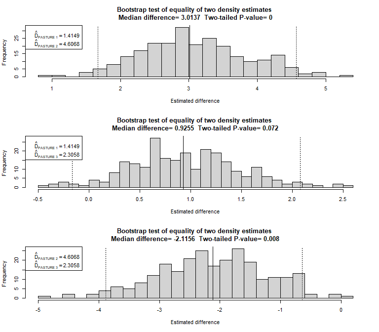
Figure 3: Two strata with Region.Label as a covariate in detection function.
Note here, when there are three strata, there are three pairwise comparisons. The function can cope with any number of strata, but recognise the number of comparisons (hence number of histograms) grows rapidly when the number of strata exceeds roughly 5.
Limitations
This function cannot compute significance of density estimate differences when estimation is carried out via multiple calls to ds(), as would be the case when analysing data from different study areas residing in different data files. However, based upon the provided code, it should be clear how to produce replicate density estimates via bootdht() and then difference them with a single line of code. Depending upon circumstances, it might also be possible to combine the two data sets into a single data file and treat them as strata which could allow use of the provided function.