| Distance.band | Frequency |
|---|---|
| 0.0-0.3 | 74 |
| 0.3-0.6 | 73 |
| 0.6-0.9 | 79 |
| 0.9-1.2 | 66 |
| 1.2-1.5 | 78 |
| 1.5-1.8 | 58 |
| 1.8-2.1 | 52 |
| 2.1-2.4 | 54 |
Line transect detection function fitting solution
Estimation of duck nest density by hand
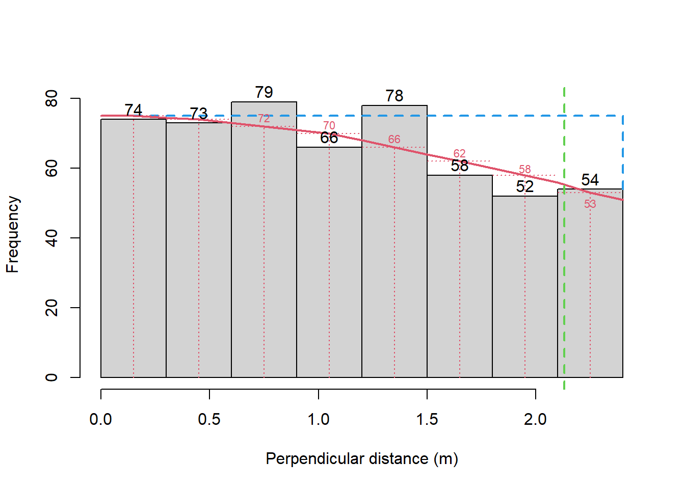
In this practical, we plot a histogram of line transect data and estimate a detection function. The data were collected during a line transect survey of duck nests in Monte Vista National Wildlife Refuge, Colorado, USA: twenty lines of 128.75 km were specified and a distance out to 2.4m was searched and the perpendicular distances of detected nests were recorded and summarised (Table 1).
- Histogram of detected nests (black) overlaid with the estimated detection function (red) is shown below.

- To estimate the area under the curve, I read off the heights of the mid points of my fitted curve (red) as follows: 75, 74, 72, 70, 66, 62, 58, 53. Therefore, my estimate of area under the curve is:
\[ Area_{curve} = (75+74+72+70+66+62+58+53) \times 0.3 = 530 \times 0.3 = 159 \] There are lots of other ways to work out the area under a curve, e.g. counting the number of grid squares under the curve on your graph paper or using the trapezoidal rule.
\[Area_{rectangle} = height \times width = 75 \times 2.4 = 180\]
Hence, my estimate of the proportion of nests detected in the covered region is:
\[\hat P_a = \frac{159}{180} = 0.883\]
- How many actual nests were there in the covered area? I saw 534 nests, and I estimate the proportion seen is 0.883, so my estimate of nests in the covered region is:
\[ \hat N_a = \frac{n}{\hat P_a} =\frac{534}{0.883} = 604.7 \textrm{ nests in the covered area}\] This estimate is for a covered area of \(a = 2wL = 2 \times (\frac{2.4}{1000}) \times 2575 = 12.36\) km\(^2\).
- I therefore estimate nest density as:
\[\hat D = \frac{\hat N_a}{2wL} = \frac{604.7}{12.36} = 48.9 \textrm{ nests per km}^2\]