Variance estimation for systematic designs
Distance for Windows exercise Solution
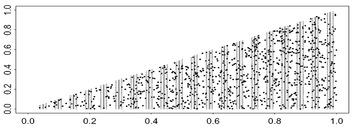
Recall the situation in which we have a strong gradient in animal density across our study region, and at the same time we also have a difference in the lengths of our transects; such that short transects are in areas of high animal density, and long transects are in areas of low animal density.

Basic variance estimation, with bootstrapping
The precision is very poor: estimated density ranges from about 1000 to 3600: a three-and-a half-fold difference over which we are uncertain. Given that our survey covered 40% of the triangle region, and had a good sample size (254 on 20 transects), this would be a very disappointing result in practice.
Bootstrap output [your results may differ slightly as these are created from a random process]:
Estimate %CV \# df 95% Confidence Interval
--------------------------------------------------------
Half-normal/Cosine
D 2129.2 27.40 999 20.74 1216.2 3727.5
                         1164.0 3427.2

Half-normal/Cosine
N 1064.6 27.40 999 20.74 608.00 1864.0
                         582.00 1714.0

Note: Confidence interval 1 uses bootstrap SE and log-normal 95% intervals.
Interval 2 is the 2.5% and 97.5% quantiles of the bootstrap estimates.
The bootstrap results are very similar to the analytic results, as we would expect. In fact, this did not used to be the case in previous versions of Distance, as the old analytic variance estimator did not perform well when there were extreme trends in both density and line length. You can access the previous default estimator under the Advanced… tab on the Variance page of the Model Definition Properties (its estimator R3), and more details are given in (Fewster et al., 2009).
The component percentages of variance are as follows:
Component Percentages of Var(D)
-------------------------------
Detection probability : 4.3
Encounter rate :       95.7
It should ring an alarm bell to see such a high contribution from Encounter rate. Generally we might expect encounter rate to be in the region of 70% to 80% for line transect surveys.
Post-stratification to improve variance estimation
- The precision is now greatly improved:
Estimate %CV df 95% Confidence Interval
-----------------------------------------------------
Half-normal/Cosine

D 2044.6 8.64 31.41 1715.0 2437.5
N 1022.0 8.64 31.41 858.00 1219.0
and a much smaller and more reasonable (considering the sample size and survey coverage) proportion of the variation comes from estimating encounter rate:
Component Percentages of Var(D)
-------------------------------
Detection probability : 44.3
Encounter rate : 55.7- The CV is now even smaller, although it could have gone either way because this is an estimator of the same quantity as the last question–just a more precise estimator.
Estimate %CV df 95% Confidence Interval
-----------------------------------------------------

Half-normal/Cosine

D 2044.6 7.97 75.87 1745.0 2395.6
N 1022.0 7.97 75.87 872.00 1198.0
The encounter rate degrees of freedom are now 19 (number of lines – 1) rather than 10 (number of post-strata) for the previous question–which is why this is a more precise estimator of the variance.
Remember we have not made any change to our data by the post-stratification; we are just getting a better estimate of the variance. In this case, the increase in precision could make a fundamental difference to the utility of the survey: it might make the difference between being able to make a management decision or not. Usually, trends will not be extreme as they are in this example, and post-stratification will not make a great difference. Such an example is shown below.
Systematic designs where post-stratification is not needed

The following simulated population does not exhibit strong trends across the survey region. Otherwise, the strip dimensions and systematic design are the same as for the previous example.
Without post-stratification: analytic output
Estimate %CV df 95% Confidence Interval
------------------------------------------------------

Half-normal/Cosine

D 1954.0 8.22 50.60 1657.3 2303.9
N 977.00 8.22 50.60 829.00 1152.0
Note: Your bootstrap results will differ slightly, as bootstrapping is a random procedure.
Estimate %CV \# df 95% Confidence Interval
--------------------------------------------------------

Half-normal/Cosine

D 1947.4 10.03 999 50.60 1592.8 2380.8
                         1565.0 2350.3

Half-normal/Cosine

N 973.69 10.03 999 50.60 796.00 1190.0
                         782.00 1175.0

Note: Confidence interval 1 uses bootstrap SE and log-normal 95% intervals.
Interval 2 is the 2.5% and 97.5% quantiles of the bootstrap estimates.
With post-stratification (non-overlapping): analytic output
Estimate %CV df 95% Confidence Interval
------------------------------------------------------

Half-normal/Cosine

D 1954.0 8.38 25.80 1645.4 2320.6
N 977.00 8.38 25.80 823.00 1160.0