Variance estimation for systematic survey designs

In the lecture describing measures of precision, we explained that systematic survey designs usually have the best variance properties, but obtaining good estimates of the variance is a difficult problem for statisticians. In this exercise, we give an example of a situation where the systematic design gives a density estimate with much better precision than a random design. This means that the usual variance estimators used in the ds function, which are based on random transect placement, are far too high. The true variance is low, but the estimated variance is high.

We will see how to implement a post-stratification scheme that enables us to get a better estimate of the variance. In Section 6, we examine another case to see that the unstratified variance estimates provided by ds are usually fine for a systematic design: things only go wrong when there are strong trends in animal density, especially when the strong trends are associated with changes in line length (e.g. the highest densities always occur on the shortest lines, or vice versa).

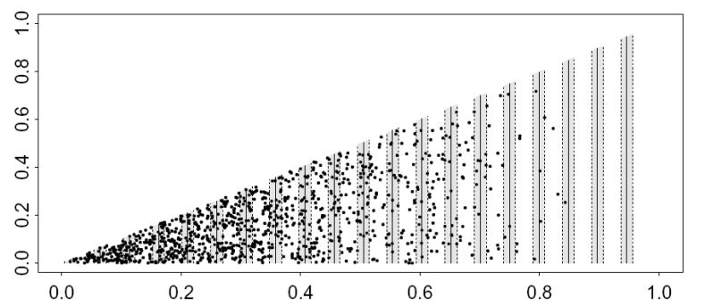
We begin with a population and survey shown below. The data used for this exercise were simulated on a computer: they are not real data. Note the characteristics for the data in Figure 1: extreme trends with very high density on short lines and very low density on long lines. Additionally, the systematic design has covered a fairly large proportion of the survey area (the covered region is shaded). These are danger signals that the usual ds variance estimators might not work well and a post-stratification scheme should be considered.

An example of survey data where there is a strong trend in density. The systematically placed search strips are shaded. Axis units are in kilometres.

Objectives

The aims of this exercise are to illustrate:

1. Default variance estimation,
2. Variance estimation with bootstrapping,
3. Post-stratification to improve variance estimation,
4. When post-stratification is not needed (optional).

Getting started

Don’t forget to load the Distance package for your session.

library(Distance)

Basic (default) variance estimation

In the code below, the necessary data file is imported and a simple model is fitted and a summary produced. Make a note of the CV of the density estimate - this is obtained using the default (analytical) estimator in the ds function and is based on the assumption that the lines were placed at random. This CV can then be compared with the CV estimates obtained from alternative methods.

# Import data
data("Systematic_variance_2")
conversion.factor <- convert_units("metre", "kilometre", "square kilometre")
# Fit a simple model
sysvar2.hn <- ds(data=Systematic_variance_2, key="hn", adjustment=NULL,
                 convert_units=conversion.factor)
# Summary
print(sysvar2.hn$dht$individuals$D)
print(sysvar2.hn$dht$individuals$N)

The true density and abundance are known (because the data were simulated): the true abundance in the survey region was \(N=1000\) and \(D=2000 \textrm{ animals per km}^2\) (i.e. 1000 animals in an area of size \(A=0.5 \textrm{km}^2\)). How do the point estimates compare with truth? What do you think about the precision of the estimates?

Variance estimation with bootstrapping

The function bootdht_Nhat_summarize pulls out the estimates of abundance \((\hat{N_i})\) for all bootstrap replicates \(i = 1, \cdots, N_{boot}\) where \(N_{boot}\) is the number of replicates requested.

The following command performs the bootstrap.

# Bootstrap estimate of uncertainty
# Run the bootstrap (this can take a while if nboot is large!) 
est.boot <- bootdht(model=sysvar2.hn, flatfile=Systematic_variance_2,
                    summary_fun=bootdht_Nhat_summarize,
                    convert_units=conversion.factor, nboot=199)

The arguments for this command are:

• model - fitted detection function model object
• flatfile - data frame of the survey data
• summary_fun - function used to obtain the summary statistics from each bootstrap
• convert_units - conversion units for abundance estimation
• nboot - number of bootstrap samples to generate. Note, it can take a long time to produce a large number of bootstraps and so perhaps try a small number at first.

# See the results
summary(est.boot)

The summary includes:

• Estimate - the median value of the bootstrap estimates
• se is the standard deviation of the bootstrap estimates
• lcl and ucl are the limits for a 95% confidence interval.
• cv is the coefficient of variation (\(CV = SE/Estimate\))

Are the bootstrapped confidence intervals for abundance and density similar to the analytical confidence intervals produced previously?

Recall that we have a particular situation in which we have systematically placed transects which are unequal in length. Furthermore, there exists an east-west gradient in animal density juxtaposed such that the shortest lines are those that pass through the portion of the study region with the highest density. In the next section, we examine a process by which we can use post-stratification to produce a better estimate of the variance in estimated abundance.

Post-stratification to improve variance estimation

The estimation of encounter rate variance in the previous section used estimators that assumed the transect lines were randomly placed throughout the triangular region. In our case, the transects were not random, but systematic and, in some circumstances, taking this in account can substantially reduce the encounter rate variance. The data we are working with is an example of this, where there are very high densities on the very shortest lines. In samples of lines, collected using a completely random design, the sample, by chance, might not contain any very short lines, or it might contain several. The variance is therefore very high, because the density estimates will be greatly affected by how many lines fall into the short-line / high-density region: we will get very low density estimates if there are no short lines, but very high density estimates if there are several short lines. By contrast, in a systematic sample, we cover the region methodically and we will always get nearly the same number of lines falling in the high density region. The systematic density variance is therefore much lower than the random placement density variance. Although there is no way of getting a variance estimate that is exactly unbiased for a systematic sample because it is effectively a sample of size 1- only the first line position was randomly chosen and the rest followed on deterministically from there. We can greatly improve on the random-based estimate by using a post-stratification scheme.

The post-stratification scheme works by grouping together pairs of adjacent lines from the systematic sample and each pair of adjacent lines is grouped into a stratum. The strata will improve variance estimation, because the systematic sample behaves more like a stratified sample than a random sample. This encounter rate estimator is called ‘O2’ (Fewster et al., 2009) and is implemented in the dht2 function.

# Post-stratification - stratified variance estimation by grouping adjacent transects

# Ensure that Sample.Labels are numeric, this is required for O2 ordering
Systematic_variance_2$Sample.Label <- as.numeric(Systematic_variance_2$Sample.Label)

# Use the Fewster et al 2009, "O2" estimator 
est.O2 <- dht2(sysvar2.hn, flatfile=Systematic_variance_2, strat_formula=~1, 
               convert_units=conversion.factor, er_est="O2")
print(est.O2, report="density")

Note that this estimator assumes that the numbering of the transects (in this example Sample.Label takes values 1 to 20) has some geographical meaning (i.e. transect 1 is next to 2 and 2 is next to 3 etc.). If this is not the case, then the user can manually define some sensible grouping of transects and create a column called grouping in the data object.

Systematic designs where post-stratification is not needed (optional)

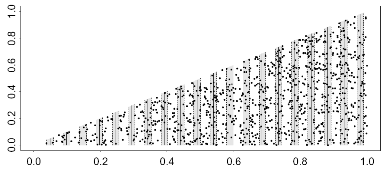
The simulated population shown in Figure 2 does not exhibit strong trends across the survey region, otherwise, the strip dimensions and systematic design are the same as for the previous example. These data are stored in the data set Systematic_variance_1.

An example of survey data that does not exhibit a trend in density. The systematically placed search strips are shaded. Axis units are in kilometres.

In the code below, these data are imported into R and a simple detection function model is fitted. The default estimate of variance is then compared to that obtained using the ‘O2’ estimator (Fewster et al., 2009).

# When post-stratification is not needed
# Import the data
data("Systematic_variance_1")
# Ensure that Sample.Labels are numeric, for O2 ordering
Systematic_variance_1$Sample.Label <- as.numeric(Systematic_variance_1$Sample.Label)
# First fit a simple model
sysvar1.hn <- ds(Systematic_variance_1, key="hn", adjustment=NULL, 
                 convert_units=conversion.factor)
# Obtain default estimates for comparison
print(sysvar1.hn$dht$individuals$D)
print(sysvar1.hn$dht$individuals$N)
# Now use Fewster et al 2009, "O2" estimator 
est1.O2 <- dht2(sysvar1.hn, flatfile=Systematic_variance_1, strat_formula=~1, 
                convert_units=conversion.factor, er_est="O2")
print(est1.O2, report="both")

Did you see a difference in the CV and 95% confidence interval between the two estimators?

References

Fewster, R. M., Buckland, S. T., Burnham, K. P., Borchers, D. L., Jupp, P. E., Laake, J. L., & Thomas, L. (2009). Estimating the encounter rate variance in distance sampling. Biometrics, 65(1), 225–236. https://doi.org/10.1111/j.1541-0420.2008.01018.x