Analysis of stratified survey data

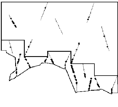
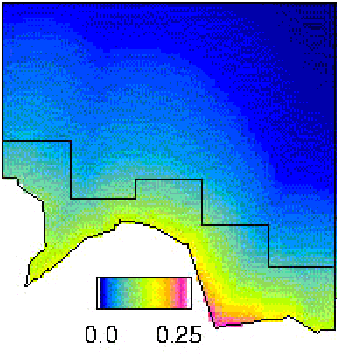
For this exercise, we use data from a survey of Antarctic minke whales. The study region was divided into two strata (North and South) the two strata were surveyed by different vessels at the same time. The minkes tend to be found in high densities against the ice edge, where they feed, and so the density in the southern stratum is typically higher than in the northern stratum (Figure 1). This is the primary reason for using a stratified survey design. It is also the reason for covering the southern stratum more intensely: in the southern stratum the transect length per unit area is more than 2.5 times that of the northern stratum.

Figure 1. An example of the sort of survey design used and a typical minke density gradient. The irregular bottom border is the ice-edge. The ‘stepped’ black line defines the boundary between the strata; dotted lines are transects and dots are detections.

Objectives

The objectives of this exercise are to:

1. Create subsets of the data
2. Decide whether to fit separate detection functions or a pooled detection function
3. Specify different stratification options using the dht2 function.

Getting started

Begin by reading in the data. Distances are in kilometers and a truncation distance of 1.5km is specified and used in the following detection function fitting. Perpendicular distances, transect lengths and study area size are all measured in kilometers; hence convert_units argument to ds is 1 and has been omitted. To keep things simple, a hazard rate detection function with no adjustments is used for all detection functions.

library(Distance)
data(minke)
head(minke)
# Specify truncation distance
minke.trunc <- 1.5

You will see that these data contain a column called ‘Region.Label’: this contains values ‘North’ or ‘South’.

Full geographical stratification

First, we want to fit encounter rate and detection function separately in each strata. This is easily performed by splitting the data by region and using ds on each subset. The commands below do this for the southern region (note, there are alternative ways to select a subset of data).

# Create dataset for South 
minke.S <- minke[minke$Region.Label=="South", ]
# Fit df to south
minke.df.S.strat <- ds(minke.S, key="hr", adjustment=NULL, truncation=minke.trunc)
summary(minke.df.S.strat)

Make a note of the AIC. Perform a similar commands to obtain estimates for the northern region. What is the total AIC?

Also make a note of the abundance in each region. What is the total abundance in the study region?

Fitting a pooled detection function

We want to compare the total AIC found previously with the AIC from fitting a detection function to all data combined. This is easy to obtain:

minke.df.all <- ds(minke, truncation=minke.trunc, key="hr", adjustment=NULL)
summary(minke.df.all)

Given the AIC value for the detection function from the pooled data, would you fit a separate detection function in each strata or not?

Stratification options using dht2

The command summary(minke.df.all) will provide the abundance estimates for each region and the total and for this simple example, this is sufficient. However, if we want to consider different stratification options, then the dht2 function is useful.

After fitting a detection function, the dht2 function, allows abundance estimates to be computed over some specified regions. In the command below, the pooled detection function is used to obtain estimates in each strata and over all (like the summary function previously used).

dht2(ddf=minke.df.all, flatfile=minke, strat_formula=~Region.Label, stratification="geographical")

The arguments are:

• ddf
  • the detection function (fitted by ds)
• flatfile
  • the data object containing all the necessary information
    • Data is referred to as being in a flatfile format if it contains information on region, transects and observations. An alternative is to use a hierarchical structure and have region, transect and observation information in separate data files with links between them to ensure that transects are mapped to the relevant region and observations to the relevant transect. We’ve not used the hierarchical structure during this workshop.
• strat_formula=~Region.Label
  • formula (hence the ~) giving the stratification structure
• stratification="geographical"
  • in this example, we specify that each strata (specified in strat_formula) represents a geographical region.
• convert_units
  • getting units conversion correct, same purpose as the convert_units argument in ds. For the minke data all measurements are in the same units, so the argument is not needed in this case.

Make a note the total abundance in the study region.

Failure to respect design during analysis

What happens if we were to ignore the regions and treat the data as though it came from one large study region? This can (dangerously) be done by changing the stratification formula, as shown below.

dht2(ddf=minke.df.all, flatfile=minke, strat_formula=~1, stratification="geographical")

Has this changed the abundance estimate? Of course it has; the question is why has this changed the abundance estimate; which estimate is proper?