  Region.Label  Area Sample.Label Effort distance object
1        South 84734            1  86.75     0.10      1
2        South 84734            1  86.75     0.22      2
3 South 84734 1 86.75 0.16 3Analysis of data from stratified surveys solution
Solution
Analysis of data from stratified surveys
Reading in the data from the stratified survey in the Southern Ocean:
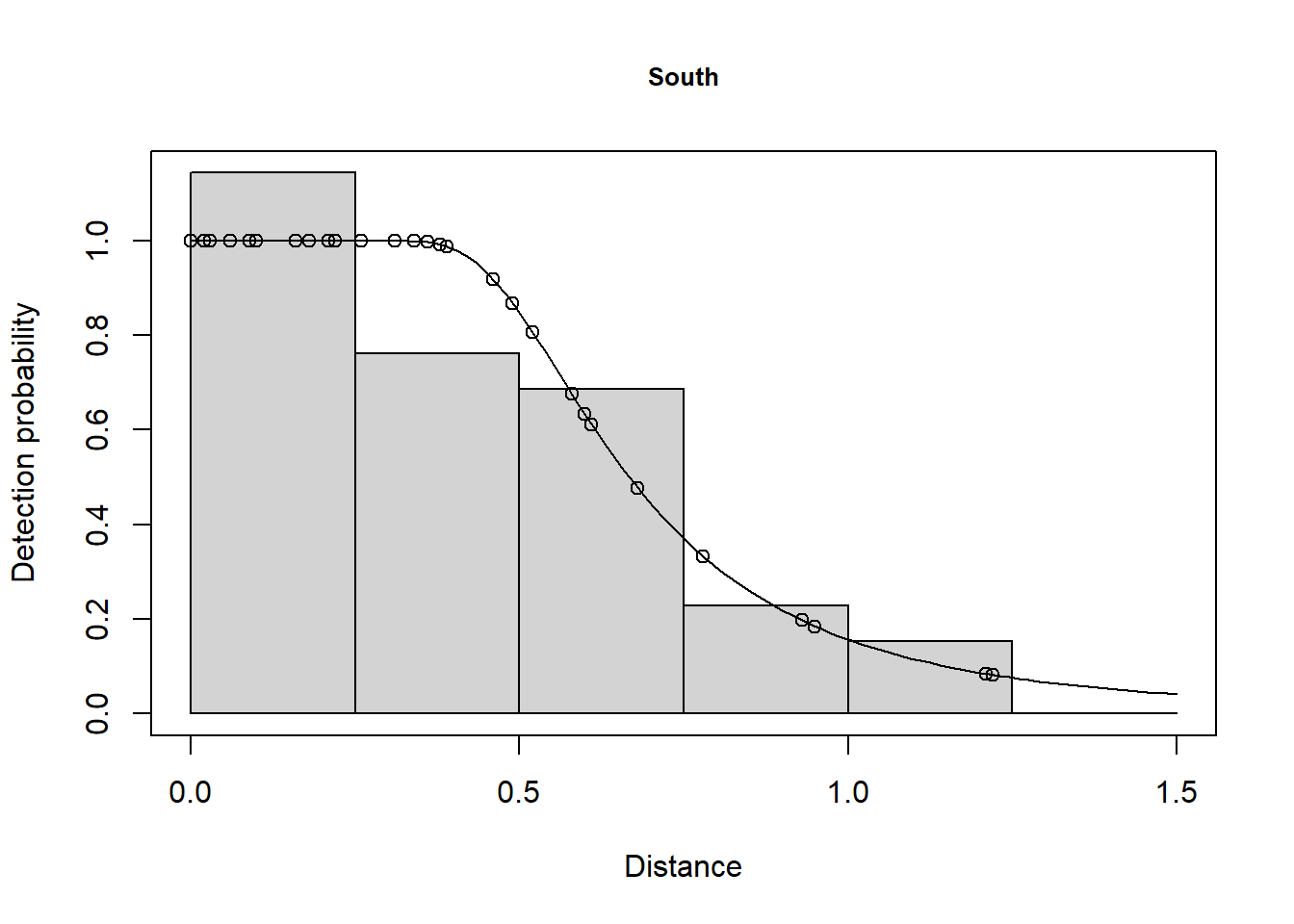
Strata treated distinctly
Fit detection function and encounter rate separately in each strata.
## Fit to each region separately - full geographical stratification
# Create data set for South
minke.S <- minke[minke$Region.Label=="South", ]
minke.df.S.strat <- ds(minke.S, truncation=minke.trunc, key="hr", adjustment=NULL)
summary(minke.df.S.strat)
Summary for distance analysis
Number of observations : 39
Distance range : 0 - 1.5
Model : Hazard-rate key function
AIC : 8.617404
Optimisation: mrds (nlminb)
Detection function parameters
Scale coefficient(s):
estimate se
(Intercept) -0.5102606 0.1921723
Shape coefficient(s):
estimate se
(Intercept) 1.242147 0.3770239
Estimate SE CV
Average p 0.4956459 0.0662961 0.133757
N in covered region 78.6852057 13.8143714 0.175565
Summary statistics:
Region Area CoveredArea Effort n k ER se.ER cv.ER
1 South 84734 1453.23 484.41 39 13 0.08051031 0.01809954 0.2248102
Abundance:
Label Estimate se cv lcl ucl df
1 Total 4587.926 1200.166 0.2615924 2687.497 7832.219 21.14052
Density:
Label Estimate se cv lcl ucl df
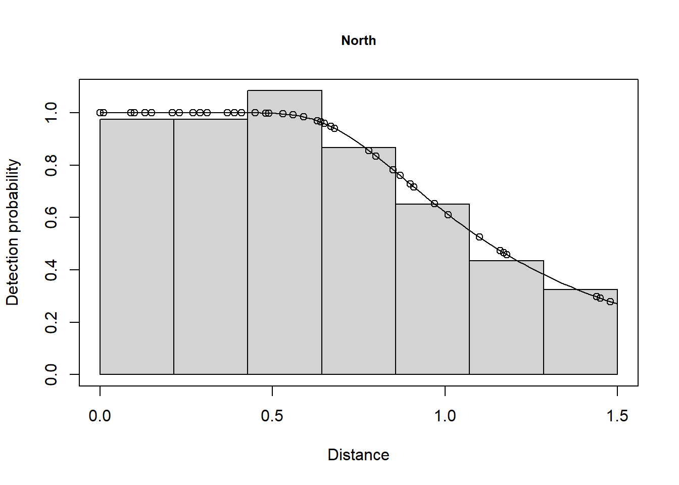
1 Total 0.05414505 0.01416393 0.2615924 0.03171687 0.09243301 21.14052# Combine selection and detection function fitting for North
minke.df.N.strat <- ds(minke[minke$Region.Label=="North", ],
truncation=minke.trunc, key="hr", adjustment=NULL)
summary(minke.df.N.strat)
Summary for distance analysis
Number of observations :  49
Distance range         :  0  -  1.5

Model       : Hazard-rate key function
AIC         :  37.27825
Optimisation:  mrds (nlminb)

Detection function parameters
Scale coefficient(s):
               estimate        se
(Intercept) -0.01081049 0.2203527

Shape coefficient(s):
            estimate        se
(Intercept) 1.022021 0.6907908

                      Estimate         SE        CV
Average p            0.7592309 0.09987677 0.1315499
N in covered region 64.5389996 9.62021709 0.1490605

Summary statistics:
  Region   Area CoveredArea  Effort  n  k         ER      se.ER     cv.ER
1  North 630582     4075.14 1358.38 49 12 0.03607238 0.01317937 0.3653591

Abundance:
  Label Estimate       se        cv      lcl     ucl       df
1 Total 9986.683 3878.032 0.3883203 4469.865 22312.5 13.98197

Density:
  Label   Estimate          se        cv         lcl        ucl       df
1 Total 0.01583725 0.006149924 0.3883203 0.007088475 0.03538397 13.98197
Detections combined across strata
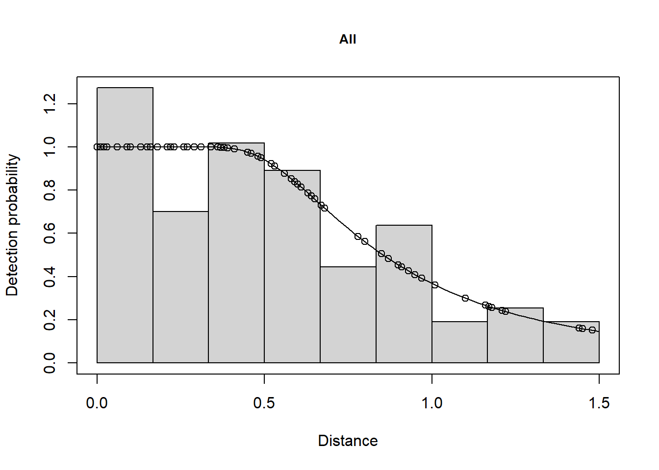
Next we fitted a pooled detection function.
Summary for distance analysis
Number of observations :  88
Distance range         :  0  -  1.5

Model       : Hazard-rate key function
AIC         :  48.63688
Optimisation:  mrds (nlminb)

Detection function parameters
Scale coefficient(s):
              estimate        se
(Intercept) -0.2967912 0.1765812

Shape coefficient(s):
             estimate        se
(Intercept) 0.9648331 0.3605009

                       Estimate         SE        CV
Average p             0.6224396  0.0668011 0.1073214
N in covered region 141.3791718 17.7757784 0.1257312

Summary statistics:
  Region   Area CoveredArea  Effort  n  k         ER      se.ER     cv.ER
1  North 630582     4075.14 1358.38 49 12 0.03607238 0.01317937 0.3653591
2  South  84734     1453.23  484.41 39 13 0.08051031 0.01809954 0.2248102
3  Total 715316     5528.37 1842.79 88 25 0.04133635 0.01181436 0.2858103

Abundance:
  Label  Estimate        se        cv      lcl       ucl       df
1 North 12181.419 4638.6283 0.3807954 5499.950 26979.692 12.96781
2 South  3653.345  910.0975 0.2491135 2181.595  6117.971 17.96263
3 Total 15834.764 4834.2848 0.3052957 8388.423 29891.167 15.25496

Density:
  Label   Estimate          se        cv         lcl        ucl       df
1 North 0.01931774 0.007356106 0.3807954 0.008722023 0.04278538 12.96781
2 South 0.04311546 0.010740641 0.2491135 0.025746391 0.07220207 17.96263
3 Total 0.02213674 0.006758251 0.3052957 0.011726878 0.04178736 15.25496
Compute combined AIC for entire study area.
Determining the correct stratification to use
The AIC value for the detection function in the South was 8.617 and the AIC for the North was 37.28. This gives a total AIC of 45.9. The AIC value for the pooled detection function was 48.64. Because 48.64 is greater than 45.9, estimation of separate detection functions in each stratum is preferable.
Differing abundance estimates from stratification decision
In the full geographical stratification, both encounter rate and detection function were estimated separately for each region (or strata). This resulted in the following abundances:
| Label | Estimate |
|---|---|
| North | 9987 |
| South | 4588 |
| Total | 14575 |
Next, the distances were combined to fit a pooled detection function but encounter rate was obtained for each region. This resulted in the following abundances:
| Label | Estimate |
|---|---|
| North | 12181 |
| South | 3653 |
| Total | 15835 |
Another approach to stratification (advanced)
An equivalent result for full geographic stratification could be produced using the dht2 function, which does not require the disaggregation of the data set into two data sets.
# Geographical stratification with stratum-specific detection function
strat.specific.detfn <- ds(data=minke, truncation=minke.trunc, key="hr",
                           adjustment=NULL, formula=~Region.Label)
abund.by.strata <- dht2(ddf=strat.specific.detfn, flatfile=minke,
                        strat_formula=~Region.Label, stratification="geographical")
print(abund.by.strata, report="abundance")
Abundance estimates from distance sampling
Stratification : geographical
Variance : R2, n/L
Multipliers : none
Sample fraction : 1
Summary statistics:
Region.Label Area CoveredArea Effort n k ER se.ER cv.ER
North 630582 4075.14 1358.38 49 12 0.036 0.013 0.365
South 84734 1453.23 484.41 39 13 0.081 0.018 0.225
Total 715316 5528.37 1842.79 88 25 0.048 0.011 0.237
Abundance estimates:
Region.Label Estimate se cv LCI UCI df
North 9865 3761.296 0.381 4451 21860 13.035
South 4651 1224.818 0.263 2719 7955 22.163
Total 14515 3970.578 0.274 8215 25648 16.065
Component percentages of variance:
Region.Label Detection ER
North 8.18 91.82
South 27.13 72.87
Total 12.49 87.51I won’t say anything just now about the wrinkle I introduced with the formula argument in the call to ds(). Recognise there is an alternative (easier) way to perform the full geographic stratification analysis without tearing apart the data. The abundance estimates presented in the last output do not identically match the estimates shown earlier for full geographic stratification, but they are close. The added benefit of this latter analysis is that the uncertainty in the total population size is computed within dht2 rather than needing to be calculated manually using the delta method.
An aside
If geographic stratification were ignored, the abundance estimate of would be 18,293 minkes. This estimate is substantially larger than the estimates above. The reason is that the survey design was geographically stratified with a smaller proportion of the north stratum receiving sampling effort and a greater proportion of the southern stratum receiving survey effort. Ignoring this inequity in the unstratified analysis would lead us to believe that the more heavily sampled southern stratum is indicative of whale density throughout the study area.